
7.1: Killing Vectors
- Page ID
- 11455

\( \newcommand{\vecs}[1]{\overset { \scriptstyle \rightharpoonup} {\mathbf{#1}} } \)
\( \newcommand{\vecd}[1]{\overset{-\!-\!\rightharpoonup}{\vphantom{a}\smash {#1}}} \)
\( \newcommand{\dsum}{\displaystyle\sum\limits} \)
\( \newcommand{\dint}{\displaystyle\int\limits} \)
\( \newcommand{\dlim}{\displaystyle\lim\limits} \)
\( \newcommand{\id}{\mathrm{id}}\) \( \newcommand{\Span}{\mathrm{span}}\)
( \newcommand{\kernel}{\mathrm{null}\,}\) \( \newcommand{\range}{\mathrm{range}\,}\)
\( \newcommand{\RealPart}{\mathrm{Re}}\) \( \newcommand{\ImaginaryPart}{\mathrm{Im}}\)
\( \newcommand{\Argument}{\mathrm{Arg}}\) \( \newcommand{\norm}[1]{\| #1 \|}\)
\( \newcommand{\inner}[2]{\langle #1, #2 \rangle}\)
\( \newcommand{\Span}{\mathrm{span}}\)
\( \newcommand{\id}{\mathrm{id}}\)
\( \newcommand{\Span}{\mathrm{span}}\)
\( \newcommand{\kernel}{\mathrm{null}\,}\)
\( \newcommand{\range}{\mathrm{range}\,}\)
\( \newcommand{\RealPart}{\mathrm{Re}}\)
\( \newcommand{\ImaginaryPart}{\mathrm{Im}}\)
\( \newcommand{\Argument}{\mathrm{Arg}}\)
\( \newcommand{\norm}[1]{\| #1 \|}\)
\( \newcommand{\inner}[2]{\langle #1, #2 \rangle}\)
\( \newcommand{\Span}{\mathrm{span}}\) \( \newcommand{\AA}{\unicode[.8,0]{x212B}}\)
\( \newcommand{\vectorA}[1]{\vec{#1}} % arrow\)
\( \newcommand{\vectorAt}[1]{\vec{\text{#1}}} % arrow\)
\( \newcommand{\vectorB}[1]{\overset { \scriptstyle \rightharpoonup} {\mathbf{#1}} } \)
\( \newcommand{\vectorC}[1]{\textbf{#1}} \)
\( \newcommand{\vectorD}[1]{\overrightarrow{#1}} \)
\( \newcommand{\vectorDt}[1]{\overrightarrow{\text{#1}}} \)
\( \newcommand{\vectE}[1]{\overset{-\!-\!\rightharpoonup}{\vphantom{a}\smash{\mathbf {#1}}}} \)
\( \newcommand{\vecs}[1]{\overset { \scriptstyle \rightharpoonup} {\mathbf{#1}} } \)
\(\newcommand{\longvect}{\overrightarrow}\)
\( \newcommand{\vecd}[1]{\overset{-\!-\!\rightharpoonup}{\vphantom{a}\smash {#1}}} \)
\(\newcommand{\avec}{\mathbf a}\) \(\newcommand{\bvec}{\mathbf b}\) \(\newcommand{\cvec}{\mathbf c}\) \(\newcommand{\dvec}{\mathbf d}\) \(\newcommand{\dtil}{\widetilde{\mathbf d}}\) \(\newcommand{\evec}{\mathbf e}\) \(\newcommand{\fvec}{\mathbf f}\) \(\newcommand{\nvec}{\mathbf n}\) \(\newcommand{\pvec}{\mathbf p}\) \(\newcommand{\qvec}{\mathbf q}\) \(\newcommand{\svec}{\mathbf s}\) \(\newcommand{\tvec}{\mathbf t}\) \(\newcommand{\uvec}{\mathbf u}\) \(\newcommand{\vvec}{\mathbf v}\) \(\newcommand{\wvec}{\mathbf w}\) \(\newcommand{\xvec}{\mathbf x}\) \(\newcommand{\yvec}{\mathbf y}\) \(\newcommand{\zvec}{\mathbf z}\) \(\newcommand{\rvec}{\mathbf r}\) \(\newcommand{\mvec}{\mathbf m}\) \(\newcommand{\zerovec}{\mathbf 0}\) \(\newcommand{\onevec}{\mathbf 1}\) \(\newcommand{\real}{\mathbb R}\) \(\newcommand{\twovec}[2]{\left[\begin{array}{r}#1 \\ #2 \end{array}\right]}\) \(\newcommand{\ctwovec}[2]{\left[\begin{array}{c}#1 \\ #2 \end{array}\right]}\) \(\newcommand{\threevec}[3]{\left[\begin{array}{r}#1 \\ #2 \\ #3 \end{array}\right]}\) \(\newcommand{\cthreevec}[3]{\left[\begin{array}{c}#1 \\ #2 \\ #3 \end{array}\right]}\) \(\newcommand{\fourvec}[4]{\left[\begin{array}{r}#1 \\ #2 \\ #3 \\ #4 \end{array}\right]}\) \(\newcommand{\cfourvec}[4]{\left[\begin{array}{c}#1 \\ #2 \\ #3 \\ #4 \end{array}\right]}\) \(\newcommand{\fivevec}[5]{\left[\begin{array}{r}#1 \\ #2 \\ #3 \\ #4 \\ #5 \\ \end{array}\right]}\) \(\newcommand{\cfivevec}[5]{\left[\begin{array}{c}#1 \\ #2 \\ #3 \\ #4 \\ #5 \\ \end{array}\right]}\) \(\newcommand{\mattwo}[4]{\left[\begin{array}{rr}#1 \amp #2 \\ #3 \amp #4 \\ \end{array}\right]}\) \(\newcommand{\laspan}[1]{\text{Span}\{#1\}}\) \(\newcommand{\bcal}{\cal B}\) \(\newcommand{\ccal}{\cal C}\) \(\newcommand{\scal}{\cal S}\) \(\newcommand{\wcal}{\cal W}\) \(\newcommand{\ecal}{\cal E}\) \(\newcommand{\coords}[2]{\left\{#1\right\}_{#2}}\) \(\newcommand{\gray}[1]{\color{gray}{#1}}\) \(\newcommand{\lgray}[1]{\color{lightgray}{#1}}\) \(\newcommand{\rank}{\operatorname{rank}}\) \(\newcommand{\row}{\text{Row}}\) \(\newcommand{\col}{\text{Col}}\) \(\renewcommand{\row}{\text{Row}}\) \(\newcommand{\nul}{\text{Nul}}\) \(\newcommand{\var}{\text{Var}}\) \(\newcommand{\corr}{\text{corr}}\) \(\newcommand{\len}[1]{\left|#1\right|}\) \(\newcommand{\bbar}{\overline{\bvec}}\) \(\newcommand{\bhat}{\widehat{\bvec}}\) \(\newcommand{\bperp}{\bvec^\perp}\) \(\newcommand{\xhat}{\widehat{\xvec}}\) \(\newcommand{\vhat}{\widehat{\vvec}}\) \(\newcommand{\uhat}{\widehat{\uvec}}\) \(\newcommand{\what}{\widehat{\wvec}}\) \(\newcommand{\Sighat}{\widehat{\Sigma}}\) \(\newcommand{\lt}{<}\) \(\newcommand{\gt}{>}\) \(\newcommand{\amp}{&}\) \(\definecolor{fillinmathshade}{gray}{0.9}\)The Schwarzschild metric is an example of a highly symmetric spacetime. It has continuous symmetries in space (under rotation) and in time (under translation in time). In addition, it has discrete symmetries under spatial reflection and time reversal. In Section 6.2, we saw that the two continuous symmetries led to the existence of conserved quantities for the trajectories of test particles, and that these could be interpreted as mass-energy and angular momentum.
Generalizing, we want to consider the idea that a metric may be invariant when every point in spacetime is systematically shifted by some infinitesimal amount. For example, the Schwarzschild metric is invariant under \(t → t + dt\). In coordinates
\[(x^0, x^1, x^2, x^3) = (t, r, \theta, \phi),\]
we have a vector field \((dt, 0, 0, 0)\) that defines the time-translation symmetry, and it is conventional to split this into two factors, a finite vector field \(\boldsymbol{\xi}\) and an infinitesimal scalar, so that the displacement vector is
\[\boldsymbol{\xi} dt = (1, 0, 0, 0) dt \ldotp\]
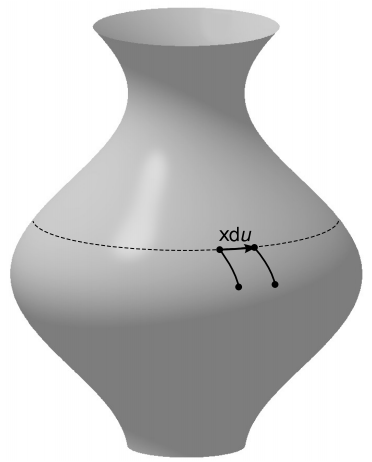
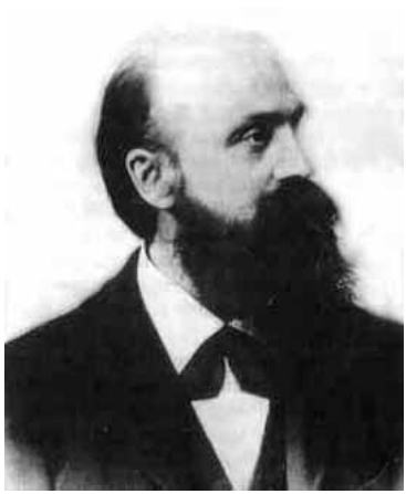
Such a field is called a Killing vector field, or simply a Killing vector, after Wilhelm Killing. When all the points in a space are displaced as specified by the Killing vector, they flow without expansion or compression. The path of a particular point, such as the dashed line in Figure \(\PageIndex{1}\), under this flow is called its orbit. Although the term “Killing vector” is singular, it refers to the entire field of vectors, each of which differs in general from the others. For example, the \(\boldsymbol{\xi}\) shown in Figure \(\PageIndex{1}\) has a greater magnitude than a \(\boldsymbol{\xi}\) near the neck of the surface.
The infinitesimal notation is designed to describe a continuous symmetry, not a discrete one. For example, the Schwarzschild spacetime also has a discrete time-reversal symmetry t → −t. This can’t be described by a Killing vector, because the displacement in time is not infinitesimal.
Example \(\PageIndex{1}\): The Euclidean plane
The Euclidean plane has two Killing vectors corresponding to translation in two linearly independent directions, plus a third Killing vector for rotation about some arbitrarily chosen origin O. In Cartesian coordinates, one way of writing a complete set of these is is
\[\begin{split} \xi_{1} &= (1, 0) \\ \xi_{2} &= (0, 1) \\ \xi_{3} &= (-y, x) \ldotp \end{split}\]
A theorem from classical geometry1 states that any transformation in the Euclidean plane that preserves distances and handedness can be expressed either as a translation or as a rotation about some point. The transformations that do not preserve handedness, such as reflections, are discrete, not continuous. This theorem tells us that there are no more Killing vectors to be found beyond these three, since any translation can be accomplished using \(\xi_{1}\) and \(\xi_{2}\), while a rotation about a point P can be done by translating P to O, rotating, and then translating O back to P.
1 Coxeter, Introduction to Geometry, ch. 3
In the example of the Schwarzschild spacetime, the components of the metric happened to be independent of t when expressed in our coordinates. This is a sufficient condition for the existence of a Killing vector, but not a necessary one. For example, it is possible to write the metric of the Euclidean plane in various forms such as
\[ds^2 = dx^2 + dy^2\]
and
\[ds^2 = dr^2 + r^2 \,d \phi^{2}.\]
The first form is independent of x and y, which demonstrates that x → x + dx and y → y + dy are Killing vectors, while the second form gives us \(\phi \rightarrow \phi + d \phi\). Although we may be able to find a particular coordinate system in which the existence of a Killing vector is manifest, its existence is an intrinsic property that holds regardless of whether we even employ coordinates. In general, we define a Killing vector not in terms of a particular system of coordinates but in purely geometrical terms: a space has a Killing vector \(\boldsymbol{\xi}\) if translation by an infinitesimal amount \(\boldsymbol{\xi}\) du doesn’t change the distance between nearby points. Statements such as “the spacetime has a timelike Killing vector” are therefore intrinsic, since both the timelike property and the property of being a Killing vector are coordinate-independent.
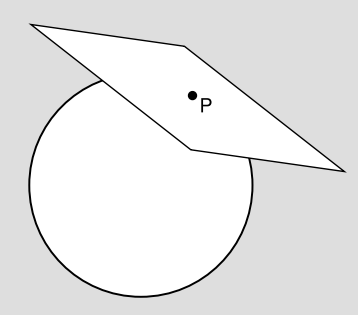
Killing vectors, like all vectors, have to live in some kind of vector space. On a manifold, this vector space is particular to a given point, Figure \(\PageIndex{3}\). A different vector space exists at every point, so that vectors at different points, occupying different spaces, can be compared only by parallel transport. Furthermore, we really have two such spaces at a given point, a space of contravariant vectors and a space of covariant ones. These are referred to as the tangent and cotangent spaces.The infinitesimal displacements we’ve been discussing belong to the contravariant (upper-index) space, but by lowering and index we can just as well discuss them as covariant vectors. The customary way of notating Killing vectors makes use of the fact, mentioned in passing in Section 5.10, that the partial derivative operators \(\partial_{0}, \partial_{1}, \partial_{2}, \partial_{3}\) form the basis for a vector space. In this notation, the Killing vector of the Schwarzschild metric we’ve been discussing can be notated simply as
\[\boldsymbol{\xi} = \partial_{t} \ldotp\]
The partial derivative notation, like the infinitesimal notation, implicitly refers to continuous symmetries rather than discrete ones. If a discrete symmetry carries a point P1 to some distant point P2, then P1 and P2 have two different tangent planes, so there is not a uniquely defined notion of whether vectors \(\boldsymbol{\xi}_{1}\) and \(\boldsymbol{\xi}_{1}\) at these two points are equal — or even approximately equal. There can therefore be no well-defined way to construe a statement such as, “P1 and P2 are separated by a displacement \(\boldsymbol{\xi}\).” In the case of a continuous symmetry, on the other hand, the two tangent planes come closer and closer to coinciding as the distance s between two points on an orbit approaches zero, and in this limit we recover an approximate notion of being able to compare vectors in the two tangent planes. They can be compared by parallel transport, and although parallel transport is path-dependent, the difference bewteen paths is proportional to the area they enclose, which varies as s2, and therefore becomes negligible in the limit s → 0.
Exercise \(\PageIndex{1}\)
Find another Killing vector of the Schwarzschild metric, and express it in the tangent-vector notation.
It can be shown that an equivalent condition for a field to be a Killing vector is
\[\nabla_{a} \boldsymbol{\xi}_{b} + \nabla_{b} \boldsymbol{\xi}_{a} = 0.\]
This relation, called the Killing equation, is written without reference to any coordinate system, in keeping with the coordinate-independence of the notion.
When a spacetime has more than one Killing vector, any linear combination of them is also a Killing vector. This means that although the existence of certain types of Killing vectors may be intrinsic, the exact choice of those vectors is not.
Example \(\PageIndex{2}\): Euclidean translations
The Euclidean plane has two translational Killing vectors (1, 0) and (0, 1), i.e., \(\partial_{x}\) and \(\partial_{y}\). These same vectors could be expressed as (1, 1) and (1, −1) in coordinate system that was rescaled and rotated by 45 degrees.
Example \(\PageIndex{3}\): a cylinder
The local properties of a cylinder, such as intrinsic flatness, are the same as the local properties of a Euclidean plane. Since the definition of a Killing vector is local and intrinsic, a cylinder has the same three Killing vectors as a plane, if we consider only a patch on the cylinder that is small enough so that it doesn’t wrap all the way around. However, only two of these — the translations — can be extended to form a smooth vector field on the entire surface of the cylinder. These might be more naturally notated in (\(\phi\), z) coordinates rather than (x, y), giving \(\partial_{z}\) and \(\partial_{\phi}\).
Example \(\PageIndex{4}\): a sphere
A sphere is like a plane or a cylinder in that it is a two-dimensional space in which no point has any properties that are intrinsically different than any other. We might expect, then, that it would have two Killing vectors. Actually it has three, \(\xi_{x} , \xi_{y}\), and \(\xi_{z}\), corresponding to infinitesimal rotations about the x, y, and z axes. To show that these are all independent Killing vectors, we need to demonstrate that we can’t, for example, have \(\xi_{x} = c_{1} \xi_{y} + c_{2} \xi_{z}\) for some constants c1 and c2. To see this, consider the actions of \(\xi_{y}\) and \(\xi_{z}\) on the point P where the x axis intersects the sphere. (References to the axes and their intersection with the sphere are extrinsic, but this is only for convenience of description and visualization.) Both \(\xi_{y}\) and \(xi_{z}\) move P around a little, and these motions are in orthogonal directions, whereas \(\xi_{x}\) leaves P fixed. This proves that we can’t have \(\xi_{x} = c_{1} \xi_{y} + c_{2} \xi_{z}\). All three Killing vectors are linearly independent.
This example shows that linear independence of Killing vectors can’t be visualized simply by thinking about the vectors in the tangent plane at one point. If that were the case, then we could have at most two linearly independent Killing vectors in this two-dimensional space. When we say “Killing vector” we’re really referring to the Killing vector field, which is defined everywhere on the space.
Example \(\PageIndex{5}\): Proving nonexistence of Killing vectors
- Find all Killing vectors of these two metrics: $$\begin{split} ds^{2} &= e^{-x} dx^{2} + e^{x} dy^{2} \\ ds^{2} &= dx^{2} + x^{2} dy^{2} \ldotp \end{split}$$
- Since both metrics are manifestly independent of y, it follows that \(\partial_{y}\) is a Killing vector for both of them. Neither one has any other manifest symmetry, so we can reasonably conjecture that this is the only Killing vector either one of them has. However, one can have symmetries that are not manifest, so it is also possible that there are more.
One way to attack this would be to use the Killing equation to find a system of differential equations, and then determine how many linearly independent solutions there were.
But there is a simpler approach. The dependence of these metrics on x suggests that the spaces may have intrinsic properties that depend on x; if so, then this demonstrates a lower symmetry than that of the Euclidean plane, which has three Killing vectors. One intrinsic property we can check is the scalar curvature R. The following Maxima code calculates R for the first metric.
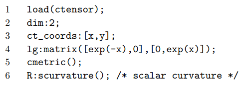
The result is R = −ex, which demonstrates that points that differ in x have different intrinsic properties. Since the flow of a Killing field \(\xi\) can never connect points that have different properties, we conclude that \(\xi_{x} = 0\). If only \(\xi_{y}\) can be nonzero, the Killing equation \(\nabla_{a} \xi_{b} + \nabla_{b} \xi_{a} = 0\) simplifies to \(\nabla_{x} \xi_{y} = \nabla_{y} \xi_{y} = 0\). These equations constrain both \(\partial_{x} \xi_{y}\) and \(\partial_{y} \xi_{y}\), which means that given a value of \(\xi_{y}\) at some point in the plane, its value everywhere else is determined. Therefore the only possible Killing vectors are scalar multiples of the Killing vector already found. Since we don’t consider Killing vectors to be distinct unless they are linearly independent, the first metric only has one Killing vector.
A similar calculation for the second metric shows that R = 0, and an explicit calculation of its Riemann tensor shows that in fact the space is flat. It is simply the Euclidean plane written in funny coordinates. This metric has the same three Killing vectors as the Euclidean plane.
It would have been tempting to leap to the wrong conclusion about the second metric by the following reasoning. The signature of a metric is an intrinsic property. The metric has signature ++ everywhere in the plane except on the y axis, where it has signature +0. This shows that the y axis has different intrinsic properties than the rest of the plane, and therefore the metric must have a lower symmetry than the Euclidean plane. It can have at most two Killing vectors, not three. This contradicts our earlier conclusion. The resolution of this paradox is that this metric has a removable degeneracy of the same type as the one described in section 6.4. As discussed in that section, the signature is invariant only under nonsingular transformations, but the transformation that converts these coordinates to Cartesian ones is singular.
Inappropriate Mixing of Notational Systems
Confusingly, it is customary to express vectors and dual vectors by summing over basis vectors like this:
\[\begin{split} \textbf{v} &= v^{\mu} \partial_{\mu} \\ \boldsymbol{\omega} &= \omega_{\mu} dx^{\mu} \ldotp \end{split}\]
This is an abuse of notation, driven by the desire to have up-down pairs of indices to sum according to the usual rules of the Einstein notation convention. But by that convention, a quantity like v or \(\boldsymbol{\omega}\) with no indices is a scalar, and that’s not the case here. The products on the right are not tensor products, i.e., the indices aren’t being contracted.
This muddle is the result of trying to make the Einstein notation do too many things at once and of trying to preserve a clumsy and outdated system of notation and terminology originated by Sylvester in 1853. In pure abstract index notation, there are not six flavors of objects as in the two equations above but only two: vectors like va and dual vectors like \(\omega_{a}\). The Sylvester notation is the prevalent one among mathematicians today, because their predecessors committed themselves to it a century before the development of alternatives like abstract index notation and birdtracks. The Sylvester system is inconsistent with the way physicists today think of vectors and dual vectors as being defined by their transformation properties, because Sylvester considers v and \(\boldsymbol{\omega}\) to be invariant.
Mixing the two systems leads to the kinds of notational clashes described above. As a particularly absurd example, a physicist who is asked to suggest a notation for a vector will typically pick up a pen and write v\(\mu\). We are then led to say that a vector is written in a concrete basis as a linear combination of dual vectors \(\partial_{\mu}\)!
Conservation Laws
Whenever a spacetime has a Killing vector, geodesics have a constant value of vb\(\xi_{b}\), where vb is the velocity four-vector. For example, because the Schwarzschild metric has a Killing vector \(\boldsymbol{\xi} = \partial_{t}\), test particles have a conserved value of vt, and therefore we also have conservation of pt, interpreted as the mass-energy.
Example \(\PageIndex{6}\): Energy-momentum in flat 1+1 spacetime
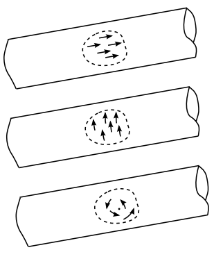
A flat 1+1-dimensional spacetime has Killing vectors \(\partial_{x}\) and \(\partial_{t}\). Corresponding to these are the conserved momentum and mass-energy, p and E. If we do a Lorentz boost, these two Killing vectors get mixed together by a linear transformation, corresponding to a transformation of p and E into a new frame.
In addition, one can define a globally conserved quantity found by integrating the flux density Pa = Tab\(\xi_{b}\) over the boundary of any compact orientable region.2 In case of a flat spacetime, there are enough Killing vectors to give conservation of energy-momentum and angular momentum.
Note
Hawking and Ellis, The Large Scale Structure of Space-Time, p. 62, give a succinct treatment that describes the flux densities and proves that Gauss’s theorem, which ordinarily fails in curved spacetime for a non-scalar flux, holds in the case where the appropriate Killing vectors exist. For an explicit description of how one can integrate to find a scalar mass-energy, see Winitzki, Topics in General Relativity, section 3.1.5, available for free online.