
3.3: Combination of Velocities
- Page ID
- 3434

\( \newcommand{\vecs}[1]{\overset { \scriptstyle \rightharpoonup} {\mathbf{#1}} } \)
\( \newcommand{\vecd}[1]{\overset{-\!-\!\rightharpoonup}{\vphantom{a}\smash {#1}}} \)
\( \newcommand{\dsum}{\displaystyle\sum\limits} \)
\( \newcommand{\dint}{\displaystyle\int\limits} \)
\( \newcommand{\dlim}{\displaystyle\lim\limits} \)
\( \newcommand{\id}{\mathrm{id}}\) \( \newcommand{\Span}{\mathrm{span}}\)
( \newcommand{\kernel}{\mathrm{null}\,}\) \( \newcommand{\range}{\mathrm{range}\,}\)
\( \newcommand{\RealPart}{\mathrm{Re}}\) \( \newcommand{\ImaginaryPart}{\mathrm{Im}}\)
\( \newcommand{\Argument}{\mathrm{Arg}}\) \( \newcommand{\norm}[1]{\| #1 \|}\)
\( \newcommand{\inner}[2]{\langle #1, #2 \rangle}\)
\( \newcommand{\Span}{\mathrm{span}}\)
\( \newcommand{\id}{\mathrm{id}}\)
\( \newcommand{\Span}{\mathrm{span}}\)
\( \newcommand{\kernel}{\mathrm{null}\,}\)
\( \newcommand{\range}{\mathrm{range}\,}\)
\( \newcommand{\RealPart}{\mathrm{Re}}\)
\( \newcommand{\ImaginaryPart}{\mathrm{Im}}\)
\( \newcommand{\Argument}{\mathrm{Arg}}\)
\( \newcommand{\norm}[1]{\| #1 \|}\)
\( \newcommand{\inner}[2]{\langle #1, #2 \rangle}\)
\( \newcommand{\Span}{\mathrm{span}}\) \( \newcommand{\AA}{\unicode[.8,0]{x212B}}\)
\( \newcommand{\vectorA}[1]{\vec{#1}} % arrow\)
\( \newcommand{\vectorAt}[1]{\vec{\text{#1}}} % arrow\)
\( \newcommand{\vectorB}[1]{\overset { \scriptstyle \rightharpoonup} {\mathbf{#1}} } \)
\( \newcommand{\vectorC}[1]{\textbf{#1}} \)
\( \newcommand{\vectorD}[1]{\overrightarrow{#1}} \)
\( \newcommand{\vectorDt}[1]{\overrightarrow{\text{#1}}} \)
\( \newcommand{\vectE}[1]{\overset{-\!-\!\rightharpoonup}{\vphantom{a}\smash{\mathbf {#1}}}} \)
\( \newcommand{\vecs}[1]{\overset { \scriptstyle \rightharpoonup} {\mathbf{#1}} } \)
\(\newcommand{\longvect}{\overrightarrow}\)
\( \newcommand{\vecd}[1]{\overset{-\!-\!\rightharpoonup}{\vphantom{a}\smash {#1}}} \)
\(\newcommand{\avec}{\mathbf a}\) \(\newcommand{\bvec}{\mathbf b}\) \(\newcommand{\cvec}{\mathbf c}\) \(\newcommand{\dvec}{\mathbf d}\) \(\newcommand{\dtil}{\widetilde{\mathbf d}}\) \(\newcommand{\evec}{\mathbf e}\) \(\newcommand{\fvec}{\mathbf f}\) \(\newcommand{\nvec}{\mathbf n}\) \(\newcommand{\pvec}{\mathbf p}\) \(\newcommand{\qvec}{\mathbf q}\) \(\newcommand{\svec}{\mathbf s}\) \(\newcommand{\tvec}{\mathbf t}\) \(\newcommand{\uvec}{\mathbf u}\) \(\newcommand{\vvec}{\mathbf v}\) \(\newcommand{\wvec}{\mathbf w}\) \(\newcommand{\xvec}{\mathbf x}\) \(\newcommand{\yvec}{\mathbf y}\) \(\newcommand{\zvec}{\mathbf z}\) \(\newcommand{\rvec}{\mathbf r}\) \(\newcommand{\mvec}{\mathbf m}\) \(\newcommand{\zerovec}{\mathbf 0}\) \(\newcommand{\onevec}{\mathbf 1}\) \(\newcommand{\real}{\mathbb R}\) \(\newcommand{\twovec}[2]{\left[\begin{array}{r}#1 \\ #2 \end{array}\right]}\) \(\newcommand{\ctwovec}[2]{\left[\begin{array}{c}#1 \\ #2 \end{array}\right]}\) \(\newcommand{\threevec}[3]{\left[\begin{array}{r}#1 \\ #2 \\ #3 \end{array}\right]}\) \(\newcommand{\cthreevec}[3]{\left[\begin{array}{c}#1 \\ #2 \\ #3 \end{array}\right]}\) \(\newcommand{\fourvec}[4]{\left[\begin{array}{r}#1 \\ #2 \\ #3 \\ #4 \end{array}\right]}\) \(\newcommand{\cfourvec}[4]{\left[\begin{array}{c}#1 \\ #2 \\ #3 \\ #4 \end{array}\right]}\) \(\newcommand{\fivevec}[5]{\left[\begin{array}{r}#1 \\ #2 \\ #3 \\ #4 \\ #5 \\ \end{array}\right]}\) \(\newcommand{\cfivevec}[5]{\left[\begin{array}{c}#1 \\ #2 \\ #3 \\ #4 \\ #5 \\ \end{array}\right]}\) \(\newcommand{\mattwo}[4]{\left[\begin{array}{rr}#1 \amp #2 \\ #3 \amp #4 \\ \end{array}\right]}\) \(\newcommand{\laspan}[1]{\text{Span}\{#1\}}\) \(\newcommand{\bcal}{\cal B}\) \(\newcommand{\ccal}{\cal C}\) \(\newcommand{\scal}{\cal S}\) \(\newcommand{\wcal}{\cal W}\) \(\newcommand{\ecal}{\cal E}\) \(\newcommand{\coords}[2]{\left\{#1\right\}_{#2}}\) \(\newcommand{\gray}[1]{\color{gray}{#1}}\) \(\newcommand{\lgray}[1]{\color{lightgray}{#1}}\) \(\newcommand{\rank}{\operatorname{rank}}\) \(\newcommand{\row}{\text{Row}}\) \(\newcommand{\col}{\text{Col}}\) \(\renewcommand{\row}{\text{Row}}\) \(\newcommand{\nul}{\text{Nul}}\) \(\newcommand{\var}{\text{Var}}\) \(\newcommand{\corr}{\text{corr}}\) \(\newcommand{\len}[1]{\left|#1\right|}\) \(\newcommand{\bbar}{\overline{\bvec}}\) \(\newcommand{\bhat}{\widehat{\bvec}}\) \(\newcommand{\bperp}{\bvec^\perp}\) \(\newcommand{\xhat}{\widehat{\xvec}}\) \(\newcommand{\vhat}{\widehat{\vvec}}\) \(\newcommand{\uhat}{\widehat{\uvec}}\) \(\newcommand{\what}{\widehat{\wvec}}\) \(\newcommand{\Sighat}{\widehat{\Sigma}}\) \(\newcommand{\lt}{<}\) \(\newcommand{\gt}{>}\) \(\newcommand{\amp}{&}\) \(\definecolor{fillinmathshade}{gray}{0.9}\)Learning Objectives
- Explain how to add velocities relativistically
In nonrelativistic physics, velocities add in relative motion. For example, if a boat moves relative to a river, and the river moves relative to the land, then the boat’s velocity relative to the land is found by vector addition. This linear behavior cannot hold relativistically. For example, if a spaceship is moving relative to the earth at velocity \(3/5\) (in units with \(c = 1\)), and it launches a probe at velocity \(3/5\) relative to itself, we can’t have the probe moving at a velocity of \(6/5\) relative to the earth, because this would be greater than the maximum speed of cause and effect, which is \(1\). To see how to add velocities relativistically, we consider the effect of carrying the two Lorentz transformations one after the other, figure \(\PageIndex{1}\).
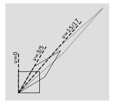
The inverse slope of the left side of each parallelogram indicates its velocity relative to the original frame, represented by the square. Since the left side of the final parallelogram has not swept past the diagonal, clearly it represents a velocity of less than \(1\), not more. To determine the result, we use the fact that the \(D\) factors multiply. We chose velocities \(3/5\) because it gives \(D = 2\), which is easy to work with. Doubling the long diagonal twice gives an over-all stretch factor of \(4\), and solving the equation \(D(v) = 4\) for \(v\) gives the result, \(v = 15/17\).
We can now see the answer to question 2 in the section 3.0: Prelude to Kinematics. If we keep accelerating a spaceship steadily, we are simply continuing the process of acceleration shown in figure \(\PageIndex{1}\). If we do this indefinitely, the velocity will approach \(c = 1\) but never surpass it. (For more on this topic of going faster than light, see section 4.7.)
Example \(\PageIndex{1}\): Accelerating electrons
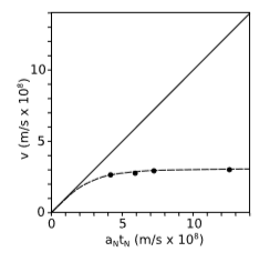
Figure \(\PageIndex{2}\) shows the results of a 1964 experiment by Bertozzi in which electrons were accelerated by the static electric field \(E\) of a Van de Graaff accelerator of length \(l_1\). They were then allowed to fly down a beamline of length \(l_2 = 8.4\) \(m\) without being acted on by any force. The time of flight \(t_2\) was used to find the final velocity \(v = \frac{l_2}{t_2}\) to which they had been accelerated. (To make the low-energy portion of the graph legible, Bertozzi’s highest energy data point is omitted.)
If we believed in Newton’s laws, then the electrons would have an acceleration
\[a_N = Ee/m\]
which would be constant if, as we pretend for the moment, the field \(E\) were constant. (The electric field inside a Van de Graaff accelerator is not really quite uniform, but this will turn out not to matter.) The Newtonian prediction for the time over which this acceleration occurs is
\[t_N = \sqrt{2ml_1/eE}\]
An acceleration \(a_N\) acting for a time \(t_N\) should produce a final velocity
\[a_Nt_N = \sqrt{2eV/m}\]
where \(V = El_1\) is the voltage difference. (By conservation of energy, this equation holds even if the field is not constant.) The solid line in the graph shows the prediction of Newton’s laws, which is that a constant force exerted steadily over time will produce a velocity that rises linearly and without limit.
The experimental data, shown as black dots, clearly tell a different story. The velocity asymptotically approaches a limit, which we identify as \(c\). The dashed line shows the predictions of special relativity, which we are not yet ready to calculate because we haven’t yet seen how kinetic energy depends on velocity at relativistic speeds.
Note that the relationship between the first and second frames of reference in figure \(\PageIndex{1}\) is the same as the relationship between the second and third. Therefore if a passenger is to feel a steady sensation of acceleration (or, equivalently, if an accelerometer aboard the ship is to show a constant reading), then the proper time required to pass from the first frame to the second must be the same as the proper time to go from the second to the third. A nice way to express this is to define the rapidity \(η = \ln D\). Combining velocities means multiplying \(D\)’s, which is the same as adding their logarithms. Therefore we can write the relativistic rule for combining velocities simply as
\[_ηc = η_1 + η_2\]
The passengers perceive the acceleration as steady if \(η\) increase by the same amount per unit of proper time. In other words, we can define a proper acceleration \(dη/dτ\), which corresponds to what an accelerometer measures.
Rapidity is convenient and useful, and is very frequently used in particle physics. But in terms of ordinary velocities, the rule for combining velocities can also be rewritten using this identity from section 3.6 as
\[v_c = \dfrac{v_1+v_2}{1+v_1v_2}. \label{eq3}\]
Exercise \(\PageIndex{1}\)
How can we tell that Equation \ref{eq3} is written in natural units? Rewrite it in SI units.