
6.6: Phase and Group Velocity
- Page ID
- 3457

\( \newcommand{\vecs}[1]{\overset { \scriptstyle \rightharpoonup} {\mathbf{#1}} } \)
\( \newcommand{\vecd}[1]{\overset{-\!-\!\rightharpoonup}{\vphantom{a}\smash {#1}}} \)
\( \newcommand{\dsum}{\displaystyle\sum\limits} \)
\( \newcommand{\dint}{\displaystyle\int\limits} \)
\( \newcommand{\dlim}{\displaystyle\lim\limits} \)
\( \newcommand{\id}{\mathrm{id}}\) \( \newcommand{\Span}{\mathrm{span}}\)
( \newcommand{\kernel}{\mathrm{null}\,}\) \( \newcommand{\range}{\mathrm{range}\,}\)
\( \newcommand{\RealPart}{\mathrm{Re}}\) \( \newcommand{\ImaginaryPart}{\mathrm{Im}}\)
\( \newcommand{\Argument}{\mathrm{Arg}}\) \( \newcommand{\norm}[1]{\| #1 \|}\)
\( \newcommand{\inner}[2]{\langle #1, #2 \rangle}\)
\( \newcommand{\Span}{\mathrm{span}}\)
\( \newcommand{\id}{\mathrm{id}}\)
\( \newcommand{\Span}{\mathrm{span}}\)
\( \newcommand{\kernel}{\mathrm{null}\,}\)
\( \newcommand{\range}{\mathrm{range}\,}\)
\( \newcommand{\RealPart}{\mathrm{Re}}\)
\( \newcommand{\ImaginaryPart}{\mathrm{Im}}\)
\( \newcommand{\Argument}{\mathrm{Arg}}\)
\( \newcommand{\norm}[1]{\| #1 \|}\)
\( \newcommand{\inner}[2]{\langle #1, #2 \rangle}\)
\( \newcommand{\Span}{\mathrm{span}}\) \( \newcommand{\AA}{\unicode[.8,0]{x212B}}\)
\( \newcommand{\vectorA}[1]{\vec{#1}} % arrow\)
\( \newcommand{\vectorAt}[1]{\vec{\text{#1}}} % arrow\)
\( \newcommand{\vectorB}[1]{\overset { \scriptstyle \rightharpoonup} {\mathbf{#1}} } \)
\( \newcommand{\vectorC}[1]{\textbf{#1}} \)
\( \newcommand{\vectorD}[1]{\overrightarrow{#1}} \)
\( \newcommand{\vectorDt}[1]{\overrightarrow{\text{#1}}} \)
\( \newcommand{\vectE}[1]{\overset{-\!-\!\rightharpoonup}{\vphantom{a}\smash{\mathbf {#1}}}} \)
\( \newcommand{\vecs}[1]{\overset { \scriptstyle \rightharpoonup} {\mathbf{#1}} } \)
\(\newcommand{\longvect}{\overrightarrow}\)
\( \newcommand{\vecd}[1]{\overset{-\!-\!\rightharpoonup}{\vphantom{a}\smash {#1}}} \)
\(\newcommand{\avec}{\mathbf a}\) \(\newcommand{\bvec}{\mathbf b}\) \(\newcommand{\cvec}{\mathbf c}\) \(\newcommand{\dvec}{\mathbf d}\) \(\newcommand{\dtil}{\widetilde{\mathbf d}}\) \(\newcommand{\evec}{\mathbf e}\) \(\newcommand{\fvec}{\mathbf f}\) \(\newcommand{\nvec}{\mathbf n}\) \(\newcommand{\pvec}{\mathbf p}\) \(\newcommand{\qvec}{\mathbf q}\) \(\newcommand{\svec}{\mathbf s}\) \(\newcommand{\tvec}{\mathbf t}\) \(\newcommand{\uvec}{\mathbf u}\) \(\newcommand{\vvec}{\mathbf v}\) \(\newcommand{\wvec}{\mathbf w}\) \(\newcommand{\xvec}{\mathbf x}\) \(\newcommand{\yvec}{\mathbf y}\) \(\newcommand{\zvec}{\mathbf z}\) \(\newcommand{\rvec}{\mathbf r}\) \(\newcommand{\mvec}{\mathbf m}\) \(\newcommand{\zerovec}{\mathbf 0}\) \(\newcommand{\onevec}{\mathbf 1}\) \(\newcommand{\real}{\mathbb R}\) \(\newcommand{\twovec}[2]{\left[\begin{array}{r}#1 \\ #2 \end{array}\right]}\) \(\newcommand{\ctwovec}[2]{\left[\begin{array}{c}#1 \\ #2 \end{array}\right]}\) \(\newcommand{\threevec}[3]{\left[\begin{array}{r}#1 \\ #2 \\ #3 \end{array}\right]}\) \(\newcommand{\cthreevec}[3]{\left[\begin{array}{c}#1 \\ #2 \\ #3 \end{array}\right]}\) \(\newcommand{\fourvec}[4]{\left[\begin{array}{r}#1 \\ #2 \\ #3 \\ #4 \end{array}\right]}\) \(\newcommand{\cfourvec}[4]{\left[\begin{array}{c}#1 \\ #2 \\ #3 \\ #4 \end{array}\right]}\) \(\newcommand{\fivevec}[5]{\left[\begin{array}{r}#1 \\ #2 \\ #3 \\ #4 \\ #5 \\ \end{array}\right]}\) \(\newcommand{\cfivevec}[5]{\left[\begin{array}{c}#1 \\ #2 \\ #3 \\ #4 \\ #5 \\ \end{array}\right]}\) \(\newcommand{\mattwo}[4]{\left[\begin{array}{rr}#1 \amp #2 \\ #3 \amp #4 \\ \end{array}\right]}\) \(\newcommand{\laspan}[1]{\text{Span}\{#1\}}\) \(\newcommand{\bcal}{\cal B}\) \(\newcommand{\ccal}{\cal C}\) \(\newcommand{\scal}{\cal S}\) \(\newcommand{\wcal}{\cal W}\) \(\newcommand{\ecal}{\cal E}\) \(\newcommand{\coords}[2]{\left\{#1\right\}_{#2}}\) \(\newcommand{\gray}[1]{\color{gray}{#1}}\) \(\newcommand{\lgray}[1]{\color{lightgray}{#1}}\) \(\newcommand{\rank}{\operatorname{rank}}\) \(\newcommand{\row}{\text{Row}}\) \(\newcommand{\col}{\text{Col}}\) \(\renewcommand{\row}{\text{Row}}\) \(\newcommand{\nul}{\text{Nul}}\) \(\newcommand{\var}{\text{Var}}\) \(\newcommand{\corr}{\text{corr}}\) \(\newcommand{\len}[1]{\left|#1\right|}\) \(\newcommand{\bbar}{\overline{\bvec}}\) \(\newcommand{\bhat}{\widehat{\bvec}}\) \(\newcommand{\bperp}{\bvec^\perp}\) \(\newcommand{\xhat}{\widehat{\xvec}}\) \(\newcommand{\vhat}{\widehat{\vvec}}\) \(\newcommand{\uhat}{\widehat{\uvec}}\) \(\newcommand{\what}{\widehat{\wvec}}\) \(\newcommand{\Sighat}{\widehat{\Sigma}}\) \(\newcommand{\lt}{<}\) \(\newcommand{\gt}{>}\) \(\newcommand{\amp}{&}\) \(\definecolor{fillinmathshade}{gray}{0.9}\)Learning Objectives
- Explain phase velocity and group velocity
Phase velocity
A wavefront is a line or surface of constant phase. In a snapshot of a wave at one moment of time, the direction of propagation of the wave is across the wavefronts. The visual situation is different in a spacetime diagram.
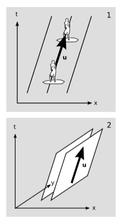
In \(1 + 1\) dimensions, figure \(\PageIndex{1}\) (1), suppose that the lines represent the crest of the water waves. The surfer is on top of a crest, riding along with it. His velocity vector \(u\) is in the spacetime direction that lies on top of the wavefront, not across it. Clearly both his motion and the propagation of the wave are to the right, not to the left as we might imagine based on experience with snapshots of waves.
In \(2+1\) dimensions, \(\PageIndex{1}\) (2), the surfer’s velocity is visualized as an arrow lying within a plane of constant phase. Given the wave’s phase information, there is more than one possible arrow of this kind. We could try to resolve the ambiguity by requiring that the arrow’s projection into the \(xy\) plane be perpendicular to the intersection of the wavefronts with that plane, but (with the exception of the case where the wave travels at \(c\), Example \(\PageIndex{1}\)) this prescription gives results that change depending on our frame of reference, and the changes are not describable by a Lorentz transformation of the velocity vector. This shows that in the general case, the phase information of the wave, encoded in the frequency covector \(ω\to \), does not describe the direction of the wave’s propagation through space. At most it tells us the wave’s phase velocity, \(ω/k\), which is not really a velocity. All of these are symptoms of the fact that a velocity is supposed to be a vector, but \(ω\to \) is a covector. The phase velocity lacks physical interest, because it is not the velocity at which any “stuff” moves.
Velocity vector of a light wave, given its phase
We’ve seen that in general, the information about the phase of a wave encoded in \(ω\to \) does not determine its direction of propagation. The exception is a wave, such as a light wave, that propagates at \(c\). Let a world-line of propagation of the wave lie along the vector \(\to v\). In the case of a wave propagating at \(c\), we have \(v^2 = 0\) (so that \(\to v\) can’t have the usual normalization for a velocity vector), and the dispersion relation is simply \(ω^2 = 0\). Since the phase stays constant along a world-line of propagation, \(ω\to v = 0\). We therefore find that \(v\) and \(ω\) are two nonzero, lightlike vectors that are orthogonal to each other. But as shown in problem Q10 in chapter 1, this implies that the two vectors are parallel. Thus if we’re given the covector \(ω\to \), we just have to compute its dual \(\to ω\) to find the direction of propagation.
Group velocity
The phase velocity is not the velocity at which “stuff” is transmitted by the wave. The velocity of the stuff is called the group velocity. To have a meaningully defined group velocity, we need to have a wave that is modulated, because an unmodulated wave is an infinite sine wave that stretches off to infinity, and such an unmodulated wave does not transmit any energy or information. An unmodulated wave has the same frequency covector \(ω\to \) throughout all of spacetime, i.e., the same frequency \(ω\) and wavenumber \(k\). One way of describing a modulated wave is by how \(ω\to \) does change.
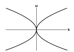
But the different components of \(ω\to \) are not free to change in any randomly chosen way. Normally they are constrained by a dispersion relation. For example, surface waves in deep water obey the constraint \(C = 0\), where \(C = ω^4 - α^2k^2\) (figure \(\PageIndex{2}\)) and \(α\) is a constant with units of acceleration, relating to the acceleration of gravity. (Since the water is infinitely deep, there is no other scale that could enter into the constraint.)
Now if a certain bump on the envelope with which the wave is modulated visits spacetime events \(P\) and \(Q\), then whatever frequency and wavelength the wave has near the bump are observed to be the same at \(P\) and \(Q\). In general, \(k\) and \(ω\) are constant along the spacetime displacement of any point on the envelope, so the spacetime displacement \(\to r\) from \(P\) to \(Q\) must satisfy the condition \((∇ω)\to r = 0\).
In addition, \(∇ω\) must be tangent to the surface of constraint \(C = 0\), so that the wave always obeys the constraint. Thus given a point \(ω\to \) in frequency space, the direction of propagation \(r\) must be uniquely determined by the constraint. Suppose \(C\) is a well-behaved function, so that it is approximately a linear function of any small change \(∆ω\), i.e., in \(1 + 1\) dimensions we have
\[\Delta C = \frac{\partial C}{\partial \omega }\Delta \omega + \frac{\partial C}{\partial k}\Delta k\]
In this approximation, \(∆C\) is a linear function that acts on a covector \(∆ω\) and gives back a scalar. In other words, \(∆C\) acts like a vector with components
\[\Delta C = \left ( \frac{\partial C}{\partial \omega }, \frac{\partial C}{\partial k} \right )\]
This vector is parallel to \(r\), so that it points in the wave’s direction of propagation through spacetime, and tells us its group velocity \(\left ( \tfrac{\partial C}{\partial k} \right )/ \left ( \tfrac{\partial C}{\partial \omega } \right )\). In our example of water waves, a calculation shows that the group velocity is \(±α/2ω\), which is half the phase velocity.