
The Multipole Expansion
- Page ID
- 11602

\( \newcommand{\vecs}[1]{\overset { \scriptstyle \rightharpoonup} {\mathbf{#1}} } \)
\( \newcommand{\vecd}[1]{\overset{-\!-\!\rightharpoonup}{\vphantom{a}\smash {#1}}} \)
\( \newcommand{\dsum}{\displaystyle\sum\limits} \)
\( \newcommand{\dint}{\displaystyle\int\limits} \)
\( \newcommand{\dlim}{\displaystyle\lim\limits} \)
\( \newcommand{\id}{\mathrm{id}}\) \( \newcommand{\Span}{\mathrm{span}}\)
( \newcommand{\kernel}{\mathrm{null}\,}\) \( \newcommand{\range}{\mathrm{range}\,}\)
\( \newcommand{\RealPart}{\mathrm{Re}}\) \( \newcommand{\ImaginaryPart}{\mathrm{Im}}\)
\( \newcommand{\Argument}{\mathrm{Arg}}\) \( \newcommand{\norm}[1]{\| #1 \|}\)
\( \newcommand{\inner}[2]{\langle #1, #2 \rangle}\)
\( \newcommand{\Span}{\mathrm{span}}\)
\( \newcommand{\id}{\mathrm{id}}\)
\( \newcommand{\Span}{\mathrm{span}}\)
\( \newcommand{\kernel}{\mathrm{null}\,}\)
\( \newcommand{\range}{\mathrm{range}\,}\)
\( \newcommand{\RealPart}{\mathrm{Re}}\)
\( \newcommand{\ImaginaryPart}{\mathrm{Im}}\)
\( \newcommand{\Argument}{\mathrm{Arg}}\)
\( \newcommand{\norm}[1]{\| #1 \|}\)
\( \newcommand{\inner}[2]{\langle #1, #2 \rangle}\)
\( \newcommand{\Span}{\mathrm{span}}\) \( \newcommand{\AA}{\unicode[.8,0]{x212B}}\)
\( \newcommand{\vectorA}[1]{\vec{#1}} % arrow\)
\( \newcommand{\vectorAt}[1]{\vec{\text{#1}}} % arrow\)
\( \newcommand{\vectorB}[1]{\overset { \scriptstyle \rightharpoonup} {\mathbf{#1}} } \)
\( \newcommand{\vectorC}[1]{\textbf{#1}} \)
\( \newcommand{\vectorD}[1]{\overrightarrow{#1}} \)
\( \newcommand{\vectorDt}[1]{\overrightarrow{\text{#1}}} \)
\( \newcommand{\vectE}[1]{\overset{-\!-\!\rightharpoonup}{\vphantom{a}\smash{\mathbf {#1}}}} \)
\( \newcommand{\vecs}[1]{\overset { \scriptstyle \rightharpoonup} {\mathbf{#1}} } \)
\(\newcommand{\longvect}{\overrightarrow}\)
\( \newcommand{\vecd}[1]{\overset{-\!-\!\rightharpoonup}{\vphantom{a}\smash {#1}}} \)
\(\newcommand{\avec}{\mathbf a}\) \(\newcommand{\bvec}{\mathbf b}\) \(\newcommand{\cvec}{\mathbf c}\) \(\newcommand{\dvec}{\mathbf d}\) \(\newcommand{\dtil}{\widetilde{\mathbf d}}\) \(\newcommand{\evec}{\mathbf e}\) \(\newcommand{\fvec}{\mathbf f}\) \(\newcommand{\nvec}{\mathbf n}\) \(\newcommand{\pvec}{\mathbf p}\) \(\newcommand{\qvec}{\mathbf q}\) \(\newcommand{\svec}{\mathbf s}\) \(\newcommand{\tvec}{\mathbf t}\) \(\newcommand{\uvec}{\mathbf u}\) \(\newcommand{\vvec}{\mathbf v}\) \(\newcommand{\wvec}{\mathbf w}\) \(\newcommand{\xvec}{\mathbf x}\) \(\newcommand{\yvec}{\mathbf y}\) \(\newcommand{\zvec}{\mathbf z}\) \(\newcommand{\rvec}{\mathbf r}\) \(\newcommand{\mvec}{\mathbf m}\) \(\newcommand{\zerovec}{\mathbf 0}\) \(\newcommand{\onevec}{\mathbf 1}\) \(\newcommand{\real}{\mathbb R}\) \(\newcommand{\twovec}[2]{\left[\begin{array}{r}#1 \\ #2 \end{array}\right]}\) \(\newcommand{\ctwovec}[2]{\left[\begin{array}{c}#1 \\ #2 \end{array}\right]}\) \(\newcommand{\threevec}[3]{\left[\begin{array}{r}#1 \\ #2 \\ #3 \end{array}\right]}\) \(\newcommand{\cthreevec}[3]{\left[\begin{array}{c}#1 \\ #2 \\ #3 \end{array}\right]}\) \(\newcommand{\fourvec}[4]{\left[\begin{array}{r}#1 \\ #2 \\ #3 \\ #4 \end{array}\right]}\) \(\newcommand{\cfourvec}[4]{\left[\begin{array}{c}#1 \\ #2 \\ #3 \\ #4 \end{array}\right]}\) \(\newcommand{\fivevec}[5]{\left[\begin{array}{r}#1 \\ #2 \\ #3 \\ #4 \\ #5 \\ \end{array}\right]}\) \(\newcommand{\cfivevec}[5]{\left[\begin{array}{c}#1 \\ #2 \\ #3 \\ #4 \\ #5 \\ \end{array}\right]}\) \(\newcommand{\mattwo}[4]{\left[\begin{array}{rr}#1 \amp #2 \\ #3 \amp #4 \\ \end{array}\right]}\) \(\newcommand{\laspan}[1]{\text{Span}\{#1\}}\) \(\newcommand{\bcal}{\cal B}\) \(\newcommand{\ccal}{\cal C}\) \(\newcommand{\scal}{\cal S}\) \(\newcommand{\wcal}{\cal W}\) \(\newcommand{\ecal}{\cal E}\) \(\newcommand{\coords}[2]{\left\{#1\right\}_{#2}}\) \(\newcommand{\gray}[1]{\color{gray}{#1}}\) \(\newcommand{\lgray}[1]{\color{lightgray}{#1}}\) \(\newcommand{\rank}{\operatorname{rank}}\) \(\newcommand{\row}{\text{Row}}\) \(\newcommand{\col}{\text{Col}}\) \(\renewcommand{\row}{\text{Row}}\) \(\newcommand{\nul}{\text{Nul}}\) \(\newcommand{\var}{\text{Var}}\) \(\newcommand{\corr}{\text{corr}}\) \(\newcommand{\len}[1]{\left|#1\right|}\) \(\newcommand{\bbar}{\overline{\bvec}}\) \(\newcommand{\bhat}{\widehat{\bvec}}\) \(\newcommand{\bperp}{\bvec^\perp}\) \(\newcommand{\xhat}{\widehat{\xvec}}\) \(\newcommand{\vhat}{\widehat{\vvec}}\) \(\newcommand{\uhat}{\widehat{\uvec}}\) \(\newcommand{\what}{\widehat{\wvec}}\) \(\newcommand{\Sighat}{\widehat{\Sigma}}\) \(\newcommand{\lt}{<}\) \(\newcommand{\gt}{>}\) \(\newcommand{\amp}{&}\) \(\definecolor{fillinmathshade}{gray}{0.9}\)A multipole expansion is a mathematical series representing a function that depends on angles—usually the two angles on a sphere. These series are useful because they can often be truncated, meaning that only the first few terms need to be retained for a good approximation to the original function. Multipole expansions are very frequently used in the study of electromagnetic and gravitational fields, where the fields at distant points are given in terms of sources in a small region. The multipole expansion with angles is often combined with an expansion in radius. Such a combination gives an expansion describing a function throughout three-dimensional space.
The multipole expansion is expressed as a sum of terms with progressively finer angular features. For example, the initial term—called the zeroth, or monopole, moment—is a constant, independent of angle. The following term—the first, or dipole, moment—varies once from positive to negative around the sphere. Higher-order terms (like the quadrupole and octupole) vary more quickly with angles. A multipole moment usually involves powers (or inverse powers) of the distance to the origin, as well as some angular dependence.
Setting up the System
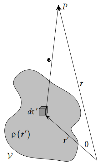
Consider an arbitrary charge distribution \( \rho (\mathbf {r} ')\). We wish to find the electrostatic potential due to this charge distribution at a given point \( \mathbf {r} \). We assume that this point is at a large distance from the charge distribution, that is if \( \mathbf {r} '\) varies over the charge distribution, then \( \mathbf {r} \gg \mathbf {r} '\).
Now, the Coulomb potential for an arbitrary charge distribution is given by
\[ V(\mathbf {r} ) ={\dfrac {1}{4\pi \epsilon _{0}}}\int _{V'}{\dfrac {\rho (\mathbf {r} ')}{|\mathbf {r} -\mathbf {r'} |}}dV' \label{eq2} \]
Here,
\[ \begin{align} | \mathbf {r} -\mathbf {r'} |&= \sqrt{ |r^{2}-2\mathbf {r} \cdot \mathbf {r} '+r'^{2}|} \\[5pt] &=r \sqrt{ \left|1-2 \dfrac {\hat {\mathbf {r}} \cdot \mathbf {r} '}{r} +\left( \dfrac {r'}{r} \right)^2 \right|} \end{align}\]
where \[ \hat {\mathbf {r} } = \mathbf {r} /r \]
Thus, using the fact that \({ \mathbf {r} }\) is much larger than \( \mathbf {r} '\), we can write
\[ \dfrac {1}{|\mathbf {r} -\mathbf {r'} |} = \dfrac {1}{r} \dfrac {1}{ \sqrt{\left|1-2 \dfrac {\hat {\mathbf {r} }\cdot \mathbf {r} '}{r} +\left(\dfrac {r'}{r}\right)^2 \right|}} \label{eq6}\]
and using the binomial expansion (see below),
\[ \dfrac {1} {\sqrt{ \left|1-2 \dfrac {\hat {\mathbf {r}} \cdot \mathbf {r} '}{r} + \left( \dfrac {r'}{r} \right)^{2} \right|} } =1-{\dfrac {\hat {\mathbf {r} }\cdot \mathbf {r} '}{r}} + {\dfrac {1}{2r^{2}}}\left(r'^{2}-3({\hat {\mathbf {r} }}\cdot \mathbf {r} '\right)^{2})+O\left({\dfrac {r'}{r}}\right)^{3} \label{eq10}\]
(we neglect the third and higher order terms).
Binomial Theorem
The binomial theory can be used to expand specific functions into an infinite series:
\[\begin{align} (1+ x )^s &= \sum_{n=0}^{\infty} \dfrac{s!}{n! (s-n)!} x^n \\[5pt] &= 1 + \dfrac{s}{1!} x + \dfrac{s(s-1)}{2!} x^2 + \dfrac{s(s-1)(s-2)}{3!} x^3 + \ldots \end{align}\]
Equation \ref{eq6} can be rewritten as
\[ \dfrac {1}{|\mathbf {r} -\mathbf {r'} |} = \dfrac {1}{r} \dfrac {1}{ \sqrt{1 + \epsilon } } \label{eq6B}\]
where
\[\epsilon = -2 \dfrac {\hat {\mathbf {r} }\cdot \mathbf {r} '}{r} +\left(\dfrac {r'}{r}\right)^2 \label{eq6c}\]
Applying the Binomial Theorem to Equation \ref{eq6B} (with \(s = -1/2\)) results in
\[ \dfrac {1}{|\mathbf {r} -\mathbf {r'} |} = \dfrac {1}{r} \left( 1 - \dfrac{1}{2} \epsilon + \dfrac{3}{8} \epsilon^2 - \dfrac{5}{16} \epsilon^3 + \ldots \right) \label{eq6d}\]
Equation \ref{eq10} originates from substituting Equation \ref{eq6c} into Equation \ref{eq6d}.
The Expansion
Inserting Equation \ref{eq10} into Equation \ref{eq2} shows that the potential can be written as
\[ V(\mathbf {r} )={\dfrac {1}{4\pi \epsilon _{0}r}}\int _{V'}\rho (\mathbf {r} ')\left(1-{\dfrac {\hat {\mathbf {r} }\cdot \mathbf {r} '}{r}}+{\dfrac {1}{2r^{2}}}\left(3({\hat {\mathbf {r} }}\cdot \mathbf {r} '\right)^{2}-r'^{2})+O\left({\dfrac {r'}{r}}\right)^{3}\right)dV' \]
We write this as
\[ V(\mathbf {r} )=V_{\text{mon}}(\mathbf {r} )+V_{\text{dip}}(\mathbf {r} )+V_{\text{quad}}(\mathbf {r} )+\ldots \label{expand}\]
The first (the zeroth-order) term in the expansion is called the monopole moment, the second (the first-order) term is called the dipole moment, the third (the second-order) is called the quadrupole moment, the fourth (third-order) term is called the octupole moment, and the fifth (fourth-order) term is called the hexadecapole moment. Given the limitation of Greek numeral prefixes, terms of higher order are conventionally named by adding "-pole" to the number of poles—e.g., 32-pole (i.e., dotriacontapole) and 64-pole (hexacontatetrapole).
These moments can be expanded thusly
\[ \begin{align} V_{\text{mon}}(\mathbf {r} ) &={\dfrac {1}{4\pi \epsilon _{0}r}}\int _{V'}\rho (\mathbf {r} ')dV' \\[5pt] V_{\text{dip}}(\mathbf {r} ) &=-{\dfrac {1}{4\pi \epsilon _{0}r^{2}}}\int _{V'}\rho (\mathbf {r} ')\left({\hat {\mathbf {r} }}\cdot \mathbf {r} '\right)dV' \\[5pt] V_{\text{quad}}(\mathbf {r} ) &={\dfrac {1}{8\pi \epsilon _{0}r^{3}}}\int _{V'}\rho (\mathbf {r} ')\left(3\left({\hat {\mathbf {r} }}\cdot \mathbf {r} '\right)^{2}-r'^{2}\right)dV' \end{align}\]
and so on.
In principle, a multipole expansion provides an exact description of the potential and generally converges under two conditions:
- if the sources (e.g. charges) are localized close to the origin and the point at which the potential is observed is far from the origin; or
- the reverse, i.e., if the sources are located far from the origin and the potential is observed close to the origin.
In the first (more common) case, the coefficients of the series expansion are called exterior multipole moments or simply multipole moments whereas, in the second case, they are called interior multipole moments.
The Monopole Scalar
Observe that
\[ V_{mon}(\mathbf {r}) =\dfrac {1}{4\pi \epsilon _0r}\int _{V'}\rho (\mathbf {r} ')dV' = \dfrac{q}{ 4\pi \epsilon _0 r}\]
is a scalar, (actually the total charge in the distribution) and is called the electric monopole. This term indicates point charge electrical potential with charge \(q\).
The Dipole Vector
If a charge distribution has a net total charge, it will tend to look like a monopole (point charge) from large distances. We can write
\[ V_{\text{dip}}(\mathbf {r} )=-{\dfrac {\hat {\mathbf {r} }}{4\pi \epsilon _{0}r^{2}}}\cdot \int _{V'}\rho (\mathbf {r} ')\mathbf {r} 'dV' \]
The vector
\[ \mathbf {p} =\int _{V'}\rho (\mathbf {r} ')\mathbf {r} 'dV' \]
is called the electric dipole. And its magnitude is called the dipole moment of the charge distribution. This terms indicates the linear charge distribution geometry of a dipole electrical potential.
The Quadrupole Tensor
Let \( \hat {\mathbf {r} }\) and \( \mathbf {r} '\) be expressed in Cartesian coordinates as \( (r_{1},r_{2},r_{3})\) and \( (x_{1},x_{2},x_{3})\). Then, \( ({\hat {\mathbf {r} }}\cdot \mathbf {r} ')^{2}=(r_{i}x_{i})^{2}=r_{i}r_{j}x_{i}x_{j}\).
We define a dyad to be the tensor \( {\hat {\mathbf {r} }}{\hat {\mathbf {r} }}\) given by
\[ \left({\hat {\mathbf {r} }}{\hat {\mathbf {r} }}\right)_{ij}=r_{i}r_{j} \]
Define the Quadrupole tensor as
\[ T=\int _{V'} \rho (\mathbf {r} ') \left(3 (\mathbf {r} '\mathbf {r} ')-\mathbf {I} r'^{2}\right)dV' \]
Then, we can write \( V_{\text{qua}}\) as the tensor contraction
\[ V_{\text{qua}}(\mathbf {r} )=- \dfrac {\hat {\mathbf {r}} \hat {\mathbf {r}}} {4\pi \epsilon _{0}r^{3}} ::T\]
this term indicates the three dimensional distribution of a quadruple electrical potential.