
6.8: Specific Heat of the Ideal Fermion Gas
- Page ID
- 18919
\( \newcommand{\vecs}[1]{\overset { \scriptstyle \rightharpoonup} {\mathbf{#1}} } \)
\( \newcommand{\vecd}[1]{\overset{-\!-\!\rightharpoonup}{\vphantom{a}\smash {#1}}} \)
\( \newcommand{\id}{\mathrm{id}}\) \( \newcommand{\Span}{\mathrm{span}}\)
( \newcommand{\kernel}{\mathrm{null}\,}\) \( \newcommand{\range}{\mathrm{range}\,}\)
\( \newcommand{\RealPart}{\mathrm{Re}}\) \( \newcommand{\ImaginaryPart}{\mathrm{Im}}\)
\( \newcommand{\Argument}{\mathrm{Arg}}\) \( \newcommand{\norm}[1]{\| #1 \|}\)
\( \newcommand{\inner}[2]{\langle #1, #2 \rangle}\)
\( \newcommand{\Span}{\mathrm{span}}\)
\( \newcommand{\id}{\mathrm{id}}\)
\( \newcommand{\Span}{\mathrm{span}}\)
\( \newcommand{\kernel}{\mathrm{null}\,}\)
\( \newcommand{\range}{\mathrm{range}\,}\)
\( \newcommand{\RealPart}{\mathrm{Re}}\)
\( \newcommand{\ImaginaryPart}{\mathrm{Im}}\)
\( \newcommand{\Argument}{\mathrm{Arg}}\)
\( \newcommand{\norm}[1]{\| #1 \|}\)
\( \newcommand{\inner}[2]{\langle #1, #2 \rangle}\)
\( \newcommand{\Span}{\mathrm{span}}\) \( \newcommand{\AA}{\unicode[.8,0]{x212B}}\)
\( \newcommand{\vectorA}[1]{\vec{#1}} % arrow\)
\( \newcommand{\vectorAt}[1]{\vec{\text{#1}}} % arrow\)
\( \newcommand{\vectorB}[1]{\overset { \scriptstyle \rightharpoonup} {\mathbf{#1}} } \)
\( \newcommand{\vectorC}[1]{\textbf{#1}} \)
\( \newcommand{\vectorD}[1]{\overrightarrow{#1}} \)
\( \newcommand{\vectorDt}[1]{\overrightarrow{\text{#1}}} \)
\( \newcommand{\vectE}[1]{\overset{-\!-\!\rightharpoonup}{\vphantom{a}\smash{\mathbf {#1}}}} \)
\( \newcommand{\vecs}[1]{\overset { \scriptstyle \rightharpoonup} {\mathbf{#1}} } \)
\( \newcommand{\vecd}[1]{\overset{-\!-\!\rightharpoonup}{\vphantom{a}\smash {#1}}} \)
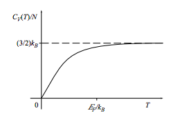
\(\newcommand{\avec}{\mathbf a}\) \(\newcommand{\bvec}{\mathbf b}\) \(\newcommand{\cvec}{\mathbf c}\) \(\newcommand{\dvec}{\mathbf d}\) \(\newcommand{\dtil}{\widetilde{\mathbf d}}\) \(\newcommand{\evec}{\mathbf e}\) \(\newcommand{\fvec}{\mathbf f}\) \(\newcommand{\nvec}{\mathbf n}\) \(\newcommand{\pvec}{\mathbf p}\) \(\newcommand{\qvec}{\mathbf q}\) \(\newcommand{\svec}{\mathbf s}\) \(\newcommand{\tvec}{\mathbf t}\) \(\newcommand{\uvec}{\mathbf u}\) \(\newcommand{\vvec}{\mathbf v}\) \(\newcommand{\wvec}{\mathbf w}\) \(\newcommand{\xvec}{\mathbf x}\) \(\newcommand{\yvec}{\mathbf y}\) \(\newcommand{\zvec}{\mathbf z}\) \(\newcommand{\rvec}{\mathbf r}\) \(\newcommand{\mvec}{\mathbf m}\) \(\newcommand{\zerovec}{\mathbf 0}\) \(\newcommand{\onevec}{\mathbf 1}\) \(\newcommand{\real}{\mathbb R}\) \(\newcommand{\twovec}[2]{\left[\begin{array}{r}#1 \\ #2 \end{array}\right]}\) \(\newcommand{\ctwovec}[2]{\left[\begin{array}{c}#1 \\ #2 \end{array}\right]}\) \(\newcommand{\threevec}[3]{\left[\begin{array}{r}#1 \\ #2 \\ #3 \end{array}\right]}\) \(\newcommand{\cthreevec}[3]{\left[\begin{array}{c}#1 \\ #2 \\ #3 \end{array}\right]}\) \(\newcommand{\fourvec}[4]{\left[\begin{array}{r}#1 \\ #2 \\ #3 \\ #4 \end{array}\right]}\) \(\newcommand{\cfourvec}[4]{\left[\begin{array}{c}#1 \\ #2 \\ #3 \\ #4 \end{array}\right]}\) \(\newcommand{\fivevec}[5]{\left[\begin{array}{r}#1 \\ #2 \\ #3 \\ #4 \\ #5 \\ \end{array}\right]}\) \(\newcommand{\cfivevec}[5]{\left[\begin{array}{c}#1 \\ #2 \\ #3 \\ #4 \\ #5 \\ \end{array}\right]}\) \(\newcommand{\mattwo}[4]{\left[\begin{array}{rr}#1 \amp #2 \\ #3 \amp #4 \\ \end{array}\right]}\) \(\newcommand{\laspan}[1]{\text{Span}\{#1\}}\) \(\newcommand{\bcal}{\cal B}\) \(\newcommand{\ccal}{\cal C}\) \(\newcommand{\scal}{\cal S}\) \(\newcommand{\wcal}{\cal W}\) \(\newcommand{\ecal}{\cal E}\) \(\newcommand{\coords}[2]{\left\{#1\right\}_{#2}}\) \(\newcommand{\gray}[1]{\color{gray}{#1}}\) \(\newcommand{\lgray}[1]{\color{lightgray}{#1}}\) \(\newcommand{\rank}{\operatorname{rank}}\) \(\newcommand{\row}{\text{Row}}\) \(\newcommand{\col}{\text{Col}}\) \(\renewcommand{\row}{\text{Row}}\) \(\newcommand{\nul}{\text{Nul}}\) \(\newcommand{\var}{\text{Var}}\) \(\newcommand{\corr}{\text{corr}}\) \(\newcommand{\len}[1]{\left|#1\right|}\) \(\newcommand{\bbar}{\overline{\bvec}}\) \(\newcommand{\bhat}{\widehat{\bvec}}\) \(\newcommand{\bperp}{\bvec^\perp}\) \(\newcommand{\xhat}{\widehat{\xvec}}\) \(\newcommand{\vhat}{\widehat{\vvec}}\) \(\newcommand{\uhat}{\widehat{\uvec}}\) \(\newcommand{\what}{\widehat{\wvec}}\) \(\newcommand{\Sighat}{\widehat{\Sigma}}\) \(\newcommand{\lt}{<}\) \(\newcommand{\gt}{>}\) \(\newcommand{\amp}{&}\) \(\definecolor{fillinmathshade}{gray}{0.9}\)There is a “set of the pants” heuristic argument showing that at low temperatures,
\[ C_{V}(T) \approx k_{B} G\left(\mathcal{E}_{F}\right)\left(k_{B} T\right).\]
This argument is not convincing in detail as far as the magnitude is concerned and, indeed, we will soon find that it is wrong by a factor of π2/3. On the other hand it is quite clear that the specific heat will increase linearly with T at low temperatures. From equipartition, the classical result is
\[ C_{V}^{\text { classical }}=\frac{3}{2} N k_{B},\]
and we expect this result to hold at high temperature. Thus our overall expectation is that the specific heat will behave as sketched below.
How can we be more precise and rigorous? That is the burden of this section.
Reminders:
\[ f(\mathcal{E})=\frac{1}{e^{(\mathcal{E}-\mu) / k_{B} T}+1}\]
\[ \mathcal{E}_{F}=\frac{\hbar^{2}}{2 m}\left(3 \pi^{2} \frac{N}{V}\right)^{2 / 3}\]
\[ G(\mathcal{E})=V \frac{\sqrt{2 m^{3}}}{\pi^{2} \hbar^{3}} \sqrt{\mathcal{E}}=N \frac{3}{2} \frac{1}{\mathcal{E}_{F}^{3 / 2}} \sqrt{\mathcal{E}}\]
The expressions for N and E are
\[ \begin{aligned} N(T, V, \mu) &=\int_{0}^{\infty} G(\mathcal{E}) f(\mathcal{E}) d \mathcal{E}=V \frac{\sqrt{2 m^{3}}}{\pi^{2} \hbar^{3}} \int_{0}^{\infty} \mathcal{E}^{1 / 2} f(\mathcal{E}) d \mathcal{E} \\ E(T, V, \mu) &=\int_{0}^{\infty} \mathcal{E} G(\mathcal{E}) f(\mathcal{E}) d \mathcal{E}=V \frac{\sqrt{2 m^{3}}}{\pi^{2} \hbar^{3}} \int_{0}^{\infty} \mathcal{E}^{3 / 2} f(\mathcal{E}) d \mathcal{E} \end{aligned}.\]
Remember how to use these expressions: The first we will invert to find µ(T, V, N), then we will plug this result into the second to find E(T, V, N). As a preliminary, recognize that we can clean up some messy expressions in terms of the physically significant constant \( \mathcal{E}_F\) by writing these two expressions as
\[ 1=\frac{3}{2} \frac{1}{\mathcal{E}_{F}^{3 / 2}} \int_{0}^{\infty} \mathcal{E}^{1 / 2} f(\mathcal{E}) d \mathcal{E}\]
\[ \frac{E}{N}=\frac{3}{2} \frac{1}{\mathcal{E}_{F}^{3 / 2}} \int_{0}^{\infty} \mathcal{E}^{3 / 2} f(\mathcal{E}) d \mathcal{E}.\]
In short, we must evaluate integrals like
\[ \int_{0}^{\infty} \frac{\mathcal{E}^{\alpha-1}}{e^{(\mathcal{E}-\mu) / k_{B} T}+1} d \mathcal{E}\]
with the dimensions of [energy]α. To make these more mathematical and less physical, convert to the dimensionless quantities
\[ x=\mathcal{E} / k_{B} T\]
\[ x_{0}=\mu / k_{B} T\]
to find
\[ \int_{0}^{\infty} \frac{\mathcal{E}^{\alpha-1}}{e^{(\mathcal{E}-\mu) / k_{B} T}+1} d \mathcal{E}=\left(k_{B} T\right)^{\alpha} \int_{0}^{\infty} \frac{x^{\alpha-1}}{e^{x-x_{0}}+1} d x.\]
Define the dimensionless integral
\[ A_{\alpha}\left(x_{0}\right)=\int_{0}^{\infty} \frac{x^{\alpha-1}}{e^{x-x_{0}}+1} d x.\]
so that
\[ 1=\frac{3}{2} \frac{\left(k_{B} T\right)^{3 / 2}}{\mathcal{E}_{F}^{3 / 2}} A_{3 / 2}\left(\mu / k_{B} T\right)\]
\[ \frac{E}{N}=\frac{3}{2} \frac{\left(k_{B} T\right)^{5 / 2}}{\mathcal{E}_{F}^{3 / 2}} A_{5 / 2}\left(\mu / k_{B} T\right).\]
Let us pause before rushing forward. You might think that we should turn to Mathematica (or to a table of integrals) and try to evaluate these integrals in terms of well-known functions like exponentials and Bessel functions. Even if we could do this, it wouldn’t help: The result would just be an incomprehensible morass of functions, and to try to understand it we would need to, among other things, look at the low-temperature limit and the high-temperature limit. Since we are particularly interested in the low-temperature behavior, let’s just set out to find the low-temperature series in the first place. The meaning of “low temperature” in this context is \(k_BT \ll \mu\) or \( x_0 = \mu /k_B T \gg 1\), so we suspect a series like
\[ E(T)=E(T=0)+\frac{E_{1}}{x_{0}}+\frac{E_{2}}{x_{0}^{2}}+\cdots.\]
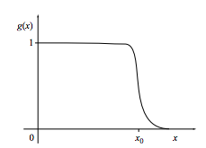
Whenever we have previously searched for such a series (for example, when we investigated internal specific heat of the rigid dumbbell, section 5.4, or the simple harmonic oscillator, problem 5.7) we had good luck using a Taylor series expansion about the origin. In this case, any such technique is doomed to failure, for the following reason: We need a good approximation for the function
\[ g(x)=\frac{1}{e^{x-x_{0}}+1},\]
a function that is very flat near the origin.
In fact, this function is so flat at the origin that, even if we kept dozens of terms in its Taylor series expansion about the origin, the Taylor approximation would be quite poor.
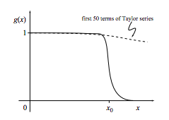
Indeed, all of the action associated with this function happens near x = x0. (We saw earlier, in our heuristic discussion, that the low-temperature specific heat was due entirely to promotion of a few electrons near the Fermi energy.) Thus an accurate low-temperature approximation will necessarily involve expansions around x = x0, not around x = 0.
Arnold Sommerfeld was aware this situation and had the genius to recognize that a change in focus would solve the problem. Specifically, the focus needs to change from the function g(x) to its derivative g'(x), because the derivative is very small for all x except near x = x0, where the action is. In specific, he noted that
\( \begin{aligned} g^{\prime}(x) &=-\frac{e^{x-x_{0}}}{\left(e^{x-x_{0}}+1\right)^{2}} \\ &=-\frac{1}{\left(e^{-\left(x-x_{0}\right) / 2}+e^{\left(x-x_{0}\right) / 2}\right)^{2}} \\ &=-\frac{1}{4 \cosh ^{2}\left(\left(x-x_{0}\right) / 2\right)} \end{aligned}.\)
The last form makes clear the remarkable fact that g'(x) is even under reflections about x0. How can we use these facts about g'(x) to solve integrals involving g(x)? Through integration by parts.
\( \begin{aligned} A_{\alpha}\left(x_{0}\right) &=\int_{0}^{\infty} x^{\alpha-1} g(x) d x \\ &=\left[\frac{x^{\alpha}}{\alpha} g(x)\right]_{0}^{\infty}-\int_{0}^{\infty} \frac{x^{\alpha}}{\alpha} g^{\prime}(x) d x \end{aligned}\)
\[ =\frac{1}{4 \alpha} \int_{0}^{\infty} \frac{x^{\alpha}}{\cosh ^{2}\left(\left(x-x_{0}\right) / 2\right)} d x\]
It’s now easy to plot the pieces of the integrand, and to see that the integrand nearly vanishes except near x = x0.
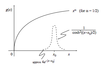
Because xα varies slowly near x = x0, it makes sense to expand it in a Taylor series about x = x0:
\( \begin{aligned} f(x) &=f\left(x_{0}\right)+f^{\prime}\left(x_{0}\right)\left(x-x_{0}\right)+\frac{1}{2} f^{\prime \prime}\left(x_{0}\right)\left(x-x_{0}\right)^{2} &+\cdots \\ x^{\alpha} &=x_{0}^{\alpha}+\alpha x_{0}^{\alpha-1}\left(x-x_{0}\right)+\frac{1}{2} \alpha(\alpha-1) x_{0}^{\alpha-2}\left(x-x_{0}\right)^{2}+\cdots \end{aligned}\)
So
\( \begin{aligned} 4 \alpha A_{\alpha}\left(x_{0}\right)=& \int_{0}^{\infty} \frac{x^{\alpha}}{\cosh ^{2}\left(\left(x-x_{0}\right) / 2\right)} d x \\=& x_{0}^{\alpha} \int_{0}^{\infty} \frac{1}{\cosh ^{2}\left(\left(x-x_{0}\right) / 2\right)} d x+\alpha x_{0}^{\alpha-1} \int_{0}^{\infty} \frac{\left(x-x_{0}\right)}{\cosh ^{2}\left(\left(x-x_{0}\right) / 2\right)} d x \\ &+\frac{1}{2} \alpha(\alpha-1) x_{0}^{\alpha-2} \int_{0}^{\infty} \frac{\left(x-x_{0}\right)^{2}}{\cosh ^{2}\left(\left(x-x_{0}\right) / 2\right)} d x+\cdots \end{aligned}.\)
Let's think about how to evaluate integrals like
\[ \int_{0}^{\infty} \frac{\left(x-x_{0}\right)^{n}}{\cosh ^{2}\left(\left(x-x_{0}\right) / 2\right)} d x.\]
The denominator is even in the variable (x − x0), while the numerator is either even or odd in the variable (x − x0). If the lower limit were −∞ instead of 0, half of these integrals would vanish. . . an immense labor savings! Now, of course, the lower limit isn’t −∞, but on the other hand if we extended the lower limit from 0 to −∞, we wouldn’t pick up much error, because the integrand nearly vanishes when x is negative. In fact, the error introduced is
\[ \int_{-\infty}^{0} \frac{\left(x-x_{0}\right)^{n}}{\cosh ^{2}\left(\left(x-x_{0}\right) / 2\right)} d x=\int_{-\infty}^{\infty} \frac{\left(x-x_{0}\right)^{n}}{\cosh ^{2}\left(\left(x-x_{0}\right) / 2\right)} d x-\int_{0}^{\infty} \frac{\left(x-x_{0}\right)^{n}}{\cosh ^{2}\left(\left(x-x_{0}\right) / 2\right)} d x ,\]
and the scale of this error is about the value of the integrand at x = 0, namely
\( \frac{\left(-x_{0}\right)^{n}}{\cosh ^{2}\left(x_{0} / 2\right)} \approx\left(-x_{0}\right)^{n}\left(4 e^{-x_{0}}\right).\)
We could find more accurate approximations for this error, but there’s no need to. We know the error is of order e−x0 and we’re interested in case that \(x_0 \gg 1\). This error is utterly negligible. Remember that we expect an answer of the form
\[ E(T)=E(T=0)+\frac{E_{1}}{x_{0}}+\frac{E_{2}}{x_{0}^{2}}+\cdots ,\]
and that (in the limit as x0 → ∞) the error e−x0 is smaller than any of these terms. . . even smaller than E492/x4920. From now on we will change the lower limit of integration from 0 to −∞, with the understanding that this replacement will introduce a negligible error. Thus, most of the remaining formulas in this section will show not equality, but rather “asymptotic equality”, denoted by the symbol ≈.
(Perhaps I’m being too glib, because while this error is indeed small, I introduce it an infinite number of times. This is the kind of problem you might want to take to your friendly neighborhood applied mathematician. These folks can usually solve the problem more easily than you can and they often appreciate your bringing neat problems to them.)
Using these ideas, we write
\( \begin{aligned} 4 \alpha A_{\alpha}\left(x_{0}\right)=& \int_{0}^{\infty} \frac{x^{\alpha}}{\cosh ^{2}\left(\left(x-x_{0}\right) / 2\right)} d x \\=& x_{0}^{\alpha} \int_{0}^{\infty} \frac{1}{\cosh ^{2}\left(\left(x-x_{0}\right) / 2\right)} d x+\alpha x_{0}^{\alpha-1} \int_{0}^{\infty} \frac{\left(x-x_{0}\right)}{\cosh ^{2}\left(\left(x-x_{0}\right) / 2\right)} d x \\ \approx & x_{0}^{\alpha} \int_{-\infty}^{\infty} \frac{1}{\cosh ^{2}\left(\left(x-x_{0}\right) / 2\right)} d x+\alpha x_{0}^{\alpha-1} \int_{-\infty}^{\infty} \frac{\left(x-x_{0}\right)}{\cosh ^{2}\left(\left(x-x_{0}\right) / 2\right)} d x \\ &+\frac{1}{2} \alpha(\alpha-1) x_{0}^{\alpha-2} \int_{-\infty}^{\infty} \frac{\left(x-x_{0}\right)^{2}}{\cosh ^{2}\left(\left(x-x_{0}\right) / 2\right)} d x+\cdots \end{aligned}\)
Because the integrals extend from −∞ to +∞, it is easy to change the variable of integration to x − x0, and then symmetry dictates that
\( \int_{-\infty}^{\infty} \frac{\left(x-x_{0}\right)^{n}}{\cosh ^{2}\left(\left(x-x_{0}\right) / 2\right)} d\left(x-x_{0}\right)=0 \quad \text { for all odd } n.\)
Using the substitution u = (x − x0)/2, we have
\[ 4 \alpha A_{\alpha}\left(x_{0}\right) \approx x_{0}^{\alpha}\left[2 \int_{-\infty}^{\infty} \frac{1}{\cosh ^{2}(u)} d u+\frac{4 \alpha(\alpha-1)}{x_{0}^{2}} \int_{-\infty}^{\infty} \frac{u^{2}}{\cosh ^{2}(u)} d u+\cdots\right]\]
The first integral can be found in Dwight and is
\( \int_{-\infty}^{\infty} \frac{1}{\cosh ^{2}(u)} d u=2.\)
The secon is Gradshteyn 3.527.5, namely
\( \int_{-\infty}^{\infty} \frac{u^{2}}{\cosh ^{2}(u)} d u=\frac{\pi^{2}}{6}.\)
Consequently
\[ A_{\alpha}\left(x_{0}\right) \approx \frac{x_{0}^{\alpha}}{\alpha}\left[1+\frac{\pi^{2}}{6} \frac{\alpha(\alpha-1)}{x_{0}^{2}}+\mathcal{O}\left(\frac{1}{x_{0}^{4}}\right)\right].\]
This is the desired series in powers of 1/x0. . . and surprisingly, all the odd powers vanish! This result is known as “the Sommerfeld expansion”.
Now we apply this formula to equation (6.106) to obtain the function µ(T):
\( \begin{aligned} 1 & \approx \frac{\mu^{3 / 2}}{\mathcal{E}_{F}^{3 / 2}}\left[1+\frac{\pi^{2}}{8}\left(\frac{k_{B} T}{\mu}\right)^{2}+\mathcal{O}\left(\frac{k_{B} T}{\mu}\right)^{4}\right] \\ \mu^{3 / 2} \approx & \mathcal{E}_{F}^{3 / 2}\left[1+\frac{\pi^{2}}{8}\left(\frac{k_{B} T}{\mu}\right)^{2}+\mathcal{O}\left(\frac{k_{B} T}{\mu}\right)^{4}\right]^{-1} \\ \mu & \approx \mathcal{E}_{F}\left[1+\frac{\pi^{2}}{8}\left(\frac{k_{B} T}{\mu}\right)^{2}+\mathcal{O}\left(\frac{k_{B} T}{\mu}\right)^{4}\right]^{-2 / 3} \\ &=\mathcal{E}_{F}\left[1-\frac{\pi^{2}}{12}\left(\frac{k_{B} T}{\mu}\right)^{2}+\mathcal{O}\left(\frac{k_{B} T}{\mu}\right)^{4}\right] \end{aligned}\)
This equation tells us a lot: It confirms that at T = 0, we have µ = \(\mathcal{E}_F\). It confirms that at T increases from zero, the chemical potential µ decreases. However it doesn’t directly give us an expression for µ(T) because µ appears on both the left and right sides. On the other hand, it does show us that µ deviates from \(\mathcal{E}_F\) by an amount proportional to (kBT/µ)2, which is small. How small?
\( \begin{aligned}\left(\frac{k_{B} T}{\mu}\right)^{2} \approx & \frac{\left(k_{B} T\right)^{2}}{\mathcal{E}_{F}^{2}\left[1-\frac{\pi^{2}}{12}\left(\frac{k_{B} T}{\mu}\right)^{2}+\mathcal{O}\left(\frac{k_{B} T}{\mu}\right)^{4}\right]^{2}} \\ &=\frac{\left(k_{B} T\right)^{2}}{\mathcal{E}_{F}^{2}\left[1-\frac{\pi^{2}}{6}\left(\frac{k_{B} T}{\mu}\right)^{2}+\mathcal{O}\left(\frac{k_{B} T}{\mu}\right)^{4}\right]} \\ &=\left(\frac{k_{B} T}{\mathcal{E}_{F}}\right)^{2}\left[1+\frac{\pi^{2}}{6}\left(\frac{k_{B} T}{\mu}\right)^{2}+\mathcal{O}\left(\frac{k_{B} T}{\mu}\right)^{4}\right] \end{aligned}\)
In other words, it is small in the sense that
\[ \left(\frac{k_{B} T}{\mu}\right)^{2} \approx\left(\frac{k_{B} T}{\mathcal{E}_{F}}\right)^{2}+\mathcal{O}\left(\frac{k_{B} T}{\mathcal{E}_{F}}\right)^{4}\]
and that
\[ \mathcal{O}\left(\frac{k_{B} T}{\mu}\right)^{4} \approx \mathcal{O}\left(\frac{k_{B} T}{\mathcal{E}_{F}}\right)^{4}\]
This gives us the desired formula for µ as a function of T:
\[ \mu(T) \approx \mathcal{E}_{F}\left[1-\frac{\pi^{2}}{12}\left(\frac{k_{B} T}{\mathcal{E}_{F}}\right)^{2}+\mathcal{O}\left(\frac{k_{B} T}{\mathcal{E}_{F}}\right)^{4}\right].\]
This result verifies our previous heuristic arguments: µ(T) declines as the temperature increases, and it does so slowly (i.e. to second order in \(k_BT/ \mathcal{E}_F\)).
Now apply expansion (6.115) for Aα to equation (6.107) to find the energy E(T, V, µ):
\[ \frac{E}{N} \approx \frac{3}{5} \frac{\mu^{5 / 2}}{\varepsilon_{F}^{3 / 2}}\left[1+\frac{5 \pi^{2}}{8}\left(\frac{k_{B} T}{\mu}\right)^{2}+\mathcal{O}\left(\frac{k_{B} T}{\mu}\right)^{4}\right].\]
Using equations (6.116) and (6.117):
\[ \frac{E}{N} \approx \frac{3}{5} \frac{\mu^{5 / 2}}{\mathcal{E}_{F}^{3 / 2}}\left[1+\frac{5 \pi^{2}}{8}\left(\frac{k_{B} T}{\mathcal{E}_{F}}\right)^{2}+\mathcal{O}\left(\frac{k_{B} T}{\mathcal{E}_{F}}\right)^{4}\right].\]
Now it’s time to plug µ(T, V, N) into E(T, V, µ) to find E(T, V, N): Use equation (6.118) for µ(T, V, N), and find
\( \mu(T)^{5 / 2} \approx \mathcal{E}_{F}^{5 / 2}\left[1-\frac{\pi^{2}}{12}\left(\frac{k_{B} T}{\mathcal{E}_{F}}\right)^{2}+\mathcal{O}\left(\frac{k_{B} T}{\mathcal{E}_{F}}\right)^{4}\right]^{5 / 2}\)
\[ =\mathcal{E}_{F}^{5 / 2}\left[1-\frac{5 \pi^{2}}{24}\left(\frac{k_{B} T}{\mathcal{E}_{F}}\right)^{2}+\mathcal{O}\left(\frac{k_{B} T}{\mathcal{E}_{F}}\right)^{4}\right].\]
Using (6.121) in (6.120) gives
\[ \frac{E}{N} \approx \frac{3}{5} \mathcal{E}_{F}\left[1-\frac{5 \pi^{2}}{24}\left(\frac{k_{B} T}{\mathcal{E}_{F}}\right)^{2}+\mathcal{O}\left(\frac{k_{B} T}{\mathcal{E}_{F}}\right)^{4}\right]\left[1+\frac{5 \pi^{2}}{8}\left(\frac{k_{B} T}{\mathcal{E}_{F}}\right)^{2}+\mathcal{O}\left(\frac{k_{B} T}{\mathcal{E}_{F}}\right)^{4}\right]\]
whence
\[ E \approx \frac{3}{5} N \mathcal{E}_{F}\left[1+\frac{5 \pi^{2}}{12}\left(\frac{k_{B} T}{\mathcal{E}_{F}}\right)^{2}+\mathcal{O}\left(\frac{k_{B} T}{\mathcal{E}_{F}}\right)^{4}\right],\]
or, for low temperatures.
\[ C_{V} \approx \frac{\pi^{2}}{2} N k_{B}\left(\frac{k_{B} T}{\mathcal{E}_{F}}\right).\]
Was all this worth it, just to get a factor of π2/3? Perhaps not, but our analysis gives us more than the factor. It gives us a better understanding of the ideal fermion gas and a deeper appreciation for the significance of the thin “action region” near \(\mathcal{E} = \mathcal{E}_F\).