10.7: G- Ramblings on the Riemann Zeta Function

The function

\( \zeta(s)=\sum_{n=1}^{\infty} \frac{1}{n^{s}} \quad \text { for } \quad s>1\)

called the Riemann zeta function, has applications to number theory, statistical mechanics, and quantal chaos.

History

From Simmons:

No great mind of the past has exerted a deeper influence on the mathematics of the twentieth century than Bernhard Riemann (1826–1866), the son of a poor country minister in northern Germany. He studied the works of Euler and Legendre while he was still in secondary school, and it is said that he mastered Legendre’s treatise on the theory of numbers in less than a week. But he was shy and modest, with little awareness of his own extraordinary abilities, so at the age of nineteen he went to the University of Göttingen with the aim of pleasing his father by studying theology and becoming a minister himself.

Instead he became a mathematician. He made contributions to the theory of complex variables (“Cauchy-Riemann equations”, “Riemann sheet”, “Riemann sphere”), to Fourier series, to analysis (“Riemann integral”), to hypergeometric functions, to convergence of infinite sums (“Riemann rearrangement theorem”), to geometry (“Riemannian curved space”), and to classical mechanics, the theory of fields and other areas of physics. In his thirties he became interested in the prime number theorem.

The first few prime numbers are 2, 3, 5, 7, 11, 13, 17, 19, 23, 29, 31, 37, 41, 43,. . . . It is clear that the primes are distributed among all the positive integers in a rather irregular way; for as we move out, they seem to occur less and less frequently, and yet there are many adjoining pairs separated by a single even number [“twin primes”]. . . . Many attempts have been made to find simple formulas for the nth prime and for the exact number of primes among the first n positive integers. All such efforts have failed, and real progress was achieved only when mathematicians started instead to look for information about the average distribution of the primes among the positive integers. It is customary to denote by π(x) the number of primes less than or equal to a positive number x. Thus π(1) = 0, π(2) = 1, π(3) = 2, π(π) = 2, π(4) = 2, and so on. In his early youth Gauss studied π(x) empirically, with the aim of finding a simple function that seems to approximate it with a small relative error for large x. On the basis of his observations he conjectured (perhaps at the age of fourteen or fifteen) that x/ log x is a good approximating function, in the sense that

\( \lim _{x \rightarrow \infty} \frac{\pi(x)}{x / \log x}=1.\)

This statement is the famous prime number theorem; and as far as anyone knows, Gauss was never able to support his guess with even a fragment of proof.

Chebyshev, unaware of Gauss’s conjecture, was the first mathematician to establish any firm conclusions about this question. In 1848 and 1850 he proved that

\( 0.9213 \ldots<\frac{\pi(x)}{x / \log x}<1.1055 \dots\)

for all sufficiently large x, and also that if the limit exists, then its value must be 1. (The numbers in the inequality are A = log 2^1/23^1/35^1/530^−1/30 on the left, and \(\frac{6}{5}A\) on the right.) . . .

In 1859 Riemann published his only work on the theory of numbers, a brief but exceedingly profound paper of less than 10 pages devoted to the prime number theorem. . . . His starting point was a remarkable identity discovered by Euler over a century earlier: if s is a real number greater than 1, then

\[ \sum_{n=1}^{\infty} \frac{1}{n^{s}}=\prod_{p} \frac{1}{1-\left(1 / p^{s}\right)},\]

where the expression on the right denotes the product of the numbers (1 − p^−s)⁻¹ for all primes p. To understand how this identity arises, we note that 1/(1 − x) = 1 + x + x 2 + · · · for |x| < 1, so for each p we have

\( \frac{1}{1-\left(1 / p^{s}\right)}=1+\frac{1}{p^{s}}+\frac{1}{p^{2 s}}+\cdots.\)

On multiplying these series for all primes p and recalling that each integer n > 1 is uniquely expressible as a product of powers of different primes, we see that

\( \begin{aligned} \prod_{p} \frac{1}{1-\left(1 / p^{s}\right)} &=\prod_{p}\left(1+\frac{1}{p^{s}}+\frac{1}{p^{2 s}}+\cdots\right) \\ &=1+\frac{1}{2^{s}}+\frac{1}{3^{s}}+\cdots+\frac{1}{n^{s}}+\cdots \\ &=\sum_{n=1}^{\infty} \frac{1}{n^{s}}\end{aligned}\)

which is the desired identity. The sum of this series is evidently a function of the real variable s > 1, and the identity establishes a connection between the behavior of this function and properties of the primes. Euler himself exploited this connection in several ways, but Riemann perceived that access to the deeper features of the distribution of primes can only be gained by allowing s to be a complex variable. . . . In his paper he proved several important properties of this function, and in a sovereign way simply stated a number of others without proof. During the century since his death, many of the finest mathematicians in the world have exerted their strongest efforts and created rich new branches of analysis in attempts to prove these statements. The first success was achieved in 1893 by J. Hadamard, and with one exception every statement has since been settled in the sense Riemann expected. (Hadamard’s work led him to his 1896 proof of the prime number theorem.) The one exception is the famous Riemann hypothesis: that all the zeros of ζ(s) in the strip 0 ≤ \(\mathcal{R}e\) ≤ 1 lie on the central line \(\mathcal{R}e {s} = \frac{1}{2}\). It stands today as the most important unsolved problem in mathematics, and is probably the most difficult problem that the mind of man has ever conceived. In a fragmentary note found among his posthumous papers, Riemann wrote that these theorems “follow from an expression for the function ζ(s) which I have not yet simplified enough to publish”. . . .

At the age of thirty-nine Riemann died of tuberculosis in Italy, on the last of several trips he undertook in order to avoid the cold, wet climate of northern Germany.

General character of the zeta function

It is easy to see that ζ(s) diverges at s = 1 and that it decreases monotonically to 1 as s increases from 1. As the historical note suggests, its behavior for complex values of s is much more elaborate.

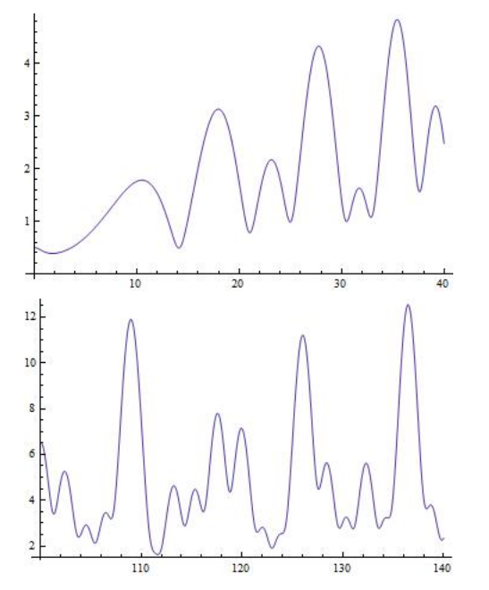
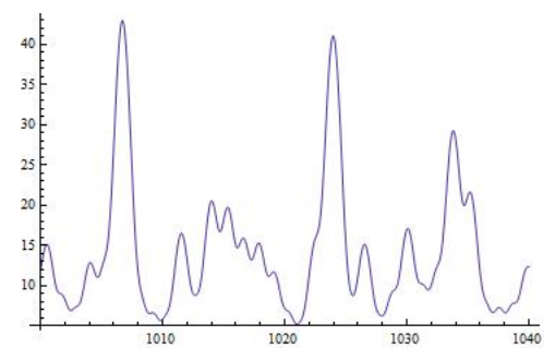
These graphs were made using Mathematica commands like

Plot[Abs[Zeta[I*y]], {y, 100, 140}].

It’s fun to try them with other values of the range.

Exact values for the zeta function

The zeta function can be evaluated exactly for positive even integer arguments:

\( \zeta(m)=\frac{(2 \pi)^{m}\left|B_{m}\right|}{2 m !} \text { for } m=2,4,6, \ldots\)

Here the B_m are the Bernoulli numbers, defined through

\( \frac{x}{e^{x}-1}=\sum_{m=0}^{\infty} \frac{B_{m}}{m !} x^{m}.\)

The first few Bernoulli numbers are

\( B_{0}=1, \quad B_{1}=-\frac{1}{2}, \quad B_{2}=\frac{1}{6}, \quad B_{4}=-\frac{1}{30}, \quad B_{6}=\frac{1}{42}, \quad B_{8}=-\frac{1}{30}, \quad B_{10}=\frac{5}{66}, \quad B_{12}=-\frac{691}{2730}\)

whence

\( \zeta(2)=\frac{\pi^{2}}{6}, \quad \zeta(4)=\frac{\pi^{4}}{90}, \quad \zeta(6)=\frac{\pi^{6}}{945}, \quad \zeta(8)=\frac{\pi^{8}}{9450}.\)

The zeta function near s = 1

The zeta function diverges with a simple pole at s = 1. In the vicinity of the divergence it is approximately equal to

\( \zeta(s) \approx C+\frac{1}{s-1}\)

where C is Euler’s constant, 0.5772. . . . (The rest of this section is stolen from Bender and Orszag.) When s is near 1, the defining series

\( \zeta(s)=\sum_{n=1}^{\infty} \frac{1}{n^{s}}\)

is very slowly converging. About 10²⁰ terms are needed to compute ζ(1.1) accurate to 1 percent!

Fortunately, there is an expression for the difference between ζ(s) and the Nth partial sum:

\( \zeta(s)=\sum_{n=0}^{N} \frac{1}{s^{n}}+\frac{1}{\Gamma(s)} \int_{0}^{\infty} \frac{u^{s-1} e^{-N u}}{e^{u}-1} d u.\)

The integral cannot be evaluated analytically but it can be expanded in an asymptotic series, giving

\[ \zeta(s) \approx \sum_{n=0}^{N} \frac{1}{s^{n}}+\frac{1}{(s-1) N^{s-1}}-\frac{1}{2 N^{s}}+\frac{B_{2} s}{N^{s+1}}+\frac{B_{4} s(s+1)(s+2)}{2 N^{s+3}}+\cdots\]

where the B_m are again the Bernoulli numbers.

Truncating this formula can give extremely accurate results. For example, using N = 9, only 38 terms of the series are needed to find ζ(1.1) accurate to 26 decimal places.

References

G.F. Simmons, Differential Equations with Applications and Historical Notes, (McGraw-Hill, New York, 1972) pp. 210–211, 214–218.

C.M. Bender and S.A. Orszag, Advanced Mathematical Methods for Scientists and Engineers, (McGraw-Hill, New York, 1978) p. 379.

Jahnke, Emde, and Lösch, Tables of Higher Functions, 6th ed. (McGraw-Hill, New York, 1960) chap. IV. (Note particularly the beautiful relief plot of |ζ(s)| for complex values of s.)

J. Spanier and K. Oldham, An Atlas of Functions, (Hemisphere Publishing, Washington, D.C., 1987) chap. 3. (Presents an algorithm purporting to find ζ(s) accurately for any real s.)

M. Abramowitz and I. Stegum, Handbook of Mathematical Functions, (National Bureau of Standards, Washington, D.C., 1964) chap. 23.

M.C. Gutzwiller, Chaos in Classical and Quantum Mechanics, (Springer-Verlag, New York, 1990) section 17.9.