10.8: H- Tutorial on Matrix Diagonalization

You know from as far back as your introductory mechanics course that some problems are difficult given one choice of coordinate axes and easy or even trivial given another. (For example, the famous “monkey and hunter” problem is difficult using a horizontal axis, but easy using an axis stretching from the hunter to the monkey.) The mathematical field of linear algebra is devoted, in large part, to systematic techniques for finding coordinate systems that make problems easy. This tutorial introduces the most valuable of these techniques. It assumes that you are familiar with matrix multiplication and with the ideas of the inverse, the transpose, and the determinant of a square matrix. It is also useful to have a nodding acquaintance with the inertia tensor.

This presentation is intentionally non-rigorous. A rigorous, formal treatment of matrix diagonalization can be found in any linear algebra textbook,¹ and there is no need to duplicate that function here. What is provided here instead is a heuristic picture of what’s going on in matrix diagonalization, how it works, and why anyone would want to do such a thing anyway. Thus this presentation complements, rather than replaces, the logically impeccable (“bulletproof”) arguments of the mathematics texts.

Essential problems in this tutorial are marked by asterisks (^*).

Warning: This tutorial is still in draft form.

H.1 What’s in a name?

There is a difference between an entity and its name. For example, a tree is made of wood, whereas its name “tree” made of ink. One way to see this is to note that in German, the name for a tree is “Baum”, so the name changes upon translation, but the tree itself does not change. (Throughout this tutorial, the term “translate” is used as in “translate from one language to another” rather than as in “translate by moving in a straight line”.)

The same holds for mathematical entities. Suppose a length is represented by the number “2” because it is two feet long. Then the same length is represented by the number “24” because it is twenty-four inches long. The same length is represented by two different numbers, just as the same tree has two different names. The representation of a length as a number depends not only upon the length, but also upon the coordinate system used to measure the length.

H.2 Vectors in two dimensions

One way of describing a two-dimensional vector V is by giving its x and y components in the form of a 2 ×1 column matrix

\[ \left(\begin{array}{l}{V_{x}} \\ {V_{y}}\end{array}\right).\]

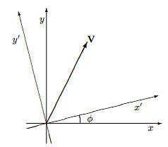
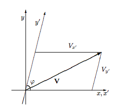
Indeed it is sometimes said that the vector V is equal to the column matrix (H.1). This is not precisely correct—it is better to say that the vector is described by the column matrix or represented by the column matrix or that its name is the column matrix. This is because if you describe the vector using a different set of coordinate axes you will come up with a different column matrix to describe the same vector. For example, in the situation shown below the descriptions in terms of the two different coordinate systems are related through the matrix equation

\[ \left(\begin{array}{c}{V_{x^{\prime}}} \\ {V_{y^{\prime}}}\end{array}\right)=\left(\begin{array}{cc}{\cos \phi} & {\sin \phi} \\ {-\sin \phi} & {\cos \phi}\end{array}\right)\left(\begin{array}{c}{V_{x}} \\ {V_{y}}\end{array}\right).\]

The 2 × 2 matrix above is called the “rotation matrix” and is usually denoted by R(ϕ):

\[ \mathrm{R}(\phi) \equiv\left(\begin{array}{cc}{\cos \phi} & {\sin \phi} \\ {-\sin \phi} & {\cos \phi}\end{array}\right)\]

One interesting property of the rotation matrix is that it is always invertible, and that its inverse is equal to its transpose. Such matrices are called orthogonal.¹ You could prove this by working a matrix multiplication, but it is easier to simply realize that the inverse of a rotation by ϕ is simply a rotation by −ϕ, and noting that

\[ \mathrm{R}^{-1}(\phi)=\mathrm{R}(-\phi)=\mathrm{R}^{\dagger}(\phi).\]

(The dagger represents matrix transposition.)

There are, of course, an infinite number of column matrix representations for any vector, corresponding to the infinite number of coordinate axis rotations with ϕ from 0 to 2π. But one of these representations is special: It is the one in which the x'-axis lines up with the vector, so the column matrix representation is just

\[ \left(\begin{array}{l}{V} \\ {0}\end{array}\right),\]

where \( V=|\mathbf{V}|=\sqrt{V_{x}^{2}+V_{y}^{2}}\) is the magnitude of the vector. This set of coordinates is the preferred (or “canonical”) set for dealing with this vector: one of the two components is zero, the easiest number to deal with, and the other component is a physically important number. You might wonder how I can claim that this representation has full information about the vector: The initial representation (H.1) contains two independent numbers, whereas the preferred representation (H.5) contains only one. The answer is that the preferred representation contains one number (the magnitude of the vector) explicitly while another number (the polar angle of the vector relative to the initial x-axis) is contained implicitly in the rotation needed to produce the preferred coordinate system.

H.1 Problem: Right angle rotations

Verify equation (H.2) in the special cases ϕ = 90^o, ϕ= 180^o, ϕ = 270^o, and ϕ = 360^o.

H.2 Problem: The rotation matrix

a. Derive equation (H.2) through purely geometrical arguments.

b. Express \(\hat{\mathbf{i}}^{\prime}\) and \(\hat{\mathbf{j}}^{\prime}\), the unit vectors of the (x', y') coordinate system, as linear combinations of \(\hat{\mathbf{i}}^{\prime}\) and \(\hat{\mathbf{j}}^{\prime}\). Then use

\[ V_{x^{\prime}}=\mathbf{V} \cdot \hat{\mathbf{i}}^{\prime} \quad \text { and } \quad V_{y^{\prime}}=\mathbf{V} \cdot \hat{\mathbf{j}}^{\prime}\]

to derive equation (H.2).

c. Which derivation do you find easier?

H.3 Problem: Rotation to the preferred coordinate system*

In the preferred coordinate system, V_y' = 0. Use this requirement to show that the preferred system is rotated from the initial system by an angle ϕ with

\[ \tan \phi=\frac{V_{y}}{V_{x}}.\]

For any value of V_y/V_x, there are two angles that satisfy this equation. What is the representation of V in each of these two coordinate systems?

H.4 Problem: A non-rotation orthogonal transformation

In one coordinate system the y-axis is vertical and the x-axis points to the right. In another the y'-axis is vertical and the x'-axis points to the left. Find the matrix that translates vector coordinates from one system to the other. Show that this matrix is orthogonal but not a rotation matrix.

H.5 Problem: Other changes of coordinate*

Suppose vertical distances (distances in the y direction) are measured in feet while horizontal distances (distances in the x direction) are measured in miles. (This system is not perverse. It is used in nearly all American road maps.) Find the matrix that changes the representation of a vector in this coordinate system to the representation of a vector in a system where all distances are measured in feet. Find the matrix that translates back. Are these matrices orthogonal?

H.6 Problem: Other special representations

At equation (H.5) we mentioned one “special” (or “canonical”) representation of a vector. There are three others, namely

\[ \left(\begin{array}{c}{0} \\ {-V}\end{array}\right), \quad\left(\begin{array}{c}{-V} \\ {0}\end{array}\right), \quad\left(\begin{array}{l}{0} \\ {V}\end{array}\right).\]

If coordinate-system rotation angle ϕ brings the vector representation into the form (H.5), then what rotation angle will result in these three representations?

H.3 Tensors in two dimensions

A tensor, like a vector, is a geometrical entity that may be described (“named”) through components, but a d-dimensional tensor requires d² rather than d components. Tensors are less familiar and more difficult to visualize than vectors, but they are neither less important nor “less physical”. We will introduce tensors through the concrete example of the inertia tensor of classical mechanics (see, for example, reference [2]), but the results we present will be perfectly general.

Just as the two components of a two-dimensional vector are most easily kept track of through a 2 × 1 matrix, so the four components of two-dimensional tensor are most conveniently written in the form of a 2×2 matrix. For example, the inertia tensor T of a point particle with mass m located² at (x, y) has components

(Note the distinction between the tensor T and its matrix of components, its “name”, T.) As with vector components, the tensor components are different in different coordinate systems, although the tensor itself does not change. For example, in the primed coordinate system of the figure on page 231, the tensor components are of course

\[ \mathrm{T}^{\prime}=\left(\begin{array}{cc}{m y^{\prime 2}} & {-m x^{\prime} y^{\prime}} \\ {-m x^{\prime} y^{\prime}} & {m x^{\prime 2}}\end{array}\right).\]

A little calculation shows that the components of the inertia tensor in two different coordinate systems are related through

\[ \mathrm{T}^{\prime}=\mathrm{R}(\phi) \mathrm{T} \mathrm{R}^{-1}(\phi).\]

This relation holds for any tensor, not just the inertia tensor. (In fact, one way to define “tensor” is as an entity with four components that satisfy the above relation under rotation.) If the matrix representing a tensor is symmetric (i.e. the matrix is equal to its transpose) in one coordinate system, then it is symmetric in all coordinate systems (see problem H.7). Therefore the symmetry is a property of the tensor, not of its matrix representation, and we may speak of “a symmetric tensor” rather than just “a tensor represented by a symmetric matrix”.

As with vectors, one of the many matrix representations of a given tensor is considered special (or “canonical”): It is the one in which the lower left component is zero. Furthermore if the tensor is symmetric (as the inertia tensor is) then in this preferred coordinate system the upper right component will be zero also, so the matrix will be all zeros except for the diagonal elements. Such a matrix is called a “diagonal matrix” and the process of finding the rotation that renders the matrix representation of a symmetric tensor diagonal is called “diagonalization”.³ We may do an “accounting of information” for this preferred coordinate system just as we did with vectors. In the initial coordinate system, the symmetric tensor had three independent components. In the preferred system, it has two independent components manifestly visible in the diagonal matrix representation, and one number hidden through the specification of the rotation.

H.7 Problem: Representations of symmetric tensors*

Show that if the matrix S representing a tensor is symmetric, and if B is any orthogonal matrix, then all of the representations

\[\mathrm{BSB}^{\dagger}\]

are symmetric. (Clue: If you try to solve this problem for rotations in two dimensions using the explicit rotation matrix (H.3), you will find it solvable but messy. The clue is that this problem asks you do prove the result in any number of dimensions, and for any orthogonal matrix B, not just rotation matrices. This more general problem is considerably easier to solve.)

H.8 Problem: Diagonal inertia tensor

The matrix (H.9) represents the inertia tensor of a point particle with mass m located a distance r from the origin. Show that the matrix is diagonal in four different coordinate systems: one in which the x'-axis points directly toward the particle, one in which the y'-axis points directly away from the particle, one in which the x'-axis points directly away from the particle, and one in which the y'-axis points directly toward the particle. Find the matrix representation in each of these four coordinate systems.

H.9 Problem: Representations of a certain tensor

Show that a tensor represented in one coordinate system by a diagonal matrix with equal elements, namely

\[ \left(\begin{array}{cc}{d_{0}} & {0} \\ {0} & {d_{0}}\end{array}\right),\]

has the same representation in all orthogonal coordinate systems.

H.10 Problem: Rotation to the preferred coordinate system*

A tensor is represented in the initial coordinate system by

\[ \left(\begin{array}{ll}{a} & {b} \\ {b} & {c}\end{array}\right).\]

Show that the tensor is diagonal in a preferred coordinate system which is rotated from the initial system by an angle ϕ with

\[ \tan (2 \phi)=\frac{2 b}{a-c}.\]

This equation has four solutions. Find the rotation matrix for ϕ = 90^o, then show how the four different diagonal representations are related. You do not need to find any of the diagonal representations in terms of a, b and c. . . just show what the other three are given that one of them is

\[ \left(\begin{array}{cc}{d_{1}} & {0} \\ {0} & {d_{2}}\end{array}\right).\]

H.11 Problem: Inertia tensor in outer product notation

The discussion in this section has emphasized the tensor’s matrix representation (“name”) T rather than the tensor T itself.

a. Define the “identity tensor” 1 as the tensor represented in some coordinate system by

\[ 1=\left(\begin{array}{ll}{1} & {0} \\ {0} & {1}\end{array}\right).\]

Show that this tensor has the same representation in any coordinate system.

b. Show that the inner product between two vectors results in a scalar: Namely

if vector bfa is represented by \(\left(\begin{array}{l}{a_{x}} \\ {a_{y}}\end{array}\right)\) and vector bfb is represented by \(\left(\begin{array}{l}{b_{x}} \\ {b_{y}}\end{array}\right)\)

then the inner product a·b is given through

\( \left(\begin{array}{cc}{a_{x}} & {a_{y}}\end{array}\right)\left(\begin{array}{c}{b_{x}} \\ {b_{y}}\end{array}\right)=a_{x} b_{x}+a_{y} b_{y}\)

and this inner product is a scalar. (A 1×2 matrix times a 2×1 matrix is a 1×1 matrix.) That is, the vector a is represented by different coordinates in different coordinate systems, and the vector b is represented by different coordinates in different coordinate systems, but the inner product a·b is the same in all coordinate systems.

c. In contrast, show that the outer product of two vectors is a tensor: Namely

\( \mathrm{ab} \doteq\left(\begin{array}{c}{a_{x}} \\ {a_{y}}\end{array}\right)\left(\begin{array}{cc}{b_{x}} & {b_{y}}\end{array}\right)=\left(\begin{array}{cc}{a_{x} b_{x}} & {a_{x} b_{y}} \\ {a_{y} b_{x}} & {a_{y} b_{y}}\end{array}\right)\)

(A 2 × 1 matrix times a 1 × 2 matrix is a 2 × 2 matrix.) That is, show that the representation of ab transforms from one coordinate system to another as specified through (H.11).

d. Show that the inertia tensor for a single particle of mass m located at position r can be written in coordinate-independent fashion as

\[ \mathbf{T}=m \mathbf{1} r^{2}-m \mathbf{r r}.\]

H.4 Tensors in three dimensions

A three-dimensional tensor is represented in component form by a 3 × 3 matrix with nine entries. If the tensor is symmetric, there are six independent elements. . . three on the diagonal and three off-diagonal. The components of a tensor in three dimensions change with coordinate system according to

\[ \mathrm{T}^{\prime}=\mathrm{RTR}^{\dagger},\]

where R is the 3 × 3 rotation matrix.

A rotation in two dimension is described completely by giving a single angle. In three dimensions more information is required. Specifically, we need not only the amount of the rotation, but we must also know the plane in which the rotation takes place. We can specify the plane by giving the unit vector perpendicular to that plane. Specifying an arbitrary vector in three dimensions requires three numbers, but specifying a unit vector in three dimensions requires only two numbers because the magnitude is already fixed at unity. Thus three numbers are required to specify a rotation in three dimensions: two to specify the rotation’s plane, one to specify the rotation’s size. (One particularly convenient way to specify a three-dimensional rotation is through the three Euler angles. Reference [3] defines these angles and shows how to write the 3 × 3 rotation matrix in terms of these variables. For the purposes of this tutorial, however, we will not need an explicit rotation matrix. . . all we need is to know is the number of angles required to specify a rotation.)

In two dimensions, any symmetric tensor (which has three independent elements), could be represented by a diagonal tensor (with two independent elements) plus a rotation (one angle). We were able to back up this claim with an explicit expression for the angle.

In three dimensions it seems reasonable that any symmetric tensor (six independent elements) can be represented by a diagonal tensor (three independent elements) plus a rotation (three angles). The three angles just have to be selected carefully enough to make sure that they cause the off-diagonal elements to vanish. This supposition is indeed correct, although we will not pause for long enough to prove it by producing explicit formulas for the three angles.

H.5 Tensors in d dimensions

A d-dimensional tensor is represented by a d×d matrix with d² entries. If the tensor is symmetric, there are d independent on-diagonal elements and d(d−1)/2 independent off-diagonal elements. The tensor components will change with coordinate system in the now-familiar form

\[ \mathrm{T}^{\prime}=\mathrm{RTR}^{\dagger},\]

where R is the d × d rotation matrix.

How many angles does it take to specify a rotation in d dimensions? Remember how we went from two dimensions to three: The three dimensional rotation took place “in a plane”, i.e. in a two-dimensional subspace. It required two (i.e. d − 1) angles to specify the orientation of the plane plus one to specify the rotation within the plane. . . a total of three angles.

A rotation in four dimensions takes place within a three-dimensional subspace. It requires 3 = d − 1 angles to specify the orientation of the three-dimensional subspace, plus, as we found above, three angles to specify the rotation within the three-dimensional subspace. . . a total of six angles.

A rotation in five dimensions requires 4 = d − 1 angles to specify the four-dimensional subspace in which the rotation occurs, plus the six angles that we have just found specify a rotation within that subspace. . . a total of ten angles.

In general, the number of angles needed to specify a rotation in d dimensions is

\[ A_{d}=d-1+A_{d-1}=d(d-1) / 2.\]

This is exactly the number of independent off-diagonal elements in a symmetric tensor. It seems reasonable that we can choose the angles to ensure that, in the resulting coordinate system, all the off-diagonal elements vanish. The proof of this result is difficult and proceeds in a very different manner from the plausibility argument sketched here. (The proof involves concepts like eigenvectors and eigenvalues, and it gives an explicit recipe for constructing the rotation matrix. It has the advantage of rigor and the disadvantage of being so technical that it’s easy to lose track of the fact that that all you’re doing is choosing a coordinate system.)

H.12 Problem: Non-symmetric tensors*

Argue that a non-symmetric tensor can be brought into a “triangular” representation in which all the elements below the diagonal are equal to zero and all the elements on and above the diagonal are independent. (This is indeed the case, although in general some of the non-zero elements remaining will be complex-valued, and some of the angles will involve rotations into complex-valued vectors.)

H.6 Linear transformations in two dimensions

Section H.3 considered 2 × 2 matrices as representations of tensors. This section gains additional insight by considering 2 × 2 matrices as representations of linear transformations. It demonstrates how diagonalization can be useful and gives a clue to an efficient algorithm for diagonalization.

A linear transformation is a function from vectors to vectors that can be represented in any given coordinate system as

\[ \left(\begin{array}{l}{u} \\ {v}\end{array}\right)=\left(\begin{array}{ll}{a_{11}} & {a_{12}} \\ {a_{21}} & {a_{22}}\end{array}\right)\left(\begin{array}{l}{x} \\ {y}\end{array}\right).\]

If the equation above represents (“names”) the transformation in one coordinate system, what is its representation in some other coordinate system? We assume that the two coordinate systems are related through an orthogonal matrix B such that

\[ \left(\begin{array}{c}{u^{\prime}} \\ {v^{\prime}}\end{array}\right)=\mathrm{B}\left(\begin{array}{l}{u} \\ {v}\end{array}\right) \quad \text { and } \quad\left(\begin{array}{c}{x^{\prime}} \\ {y^{\prime}}\end{array}\right)=\mathrm{B}\left(\begin{array}{l}{x} \\ {y}\end{array}\right).\]

(For example, if the new coordinate system is the primed coordinate system of the figure on page 231, then the matrix B that translates from the original to the new coordinates is the rotation matrix R(ϕ).) Given this “translation dictionary”, we have

\[ \left(\begin{array}{c}{u^{\prime}} \\ {v^{\prime}}\end{array}\right)=\mathrm{B}\left(\begin{array}{ll}{a_{11}} & {a_{12}} \\ {a_{21}} & {a_{22}}\end{array}\right)\left(\begin{array}{l}{x} \\ {y}\end{array}\right).\]

But B is invertible, so

\[ \left(\begin{array}{l}{x} \\ {y}\end{array}\right)=B^{-1}\left(\begin{array}{l}{x^{\prime}} \\ {y^{\prime}}\end{array}\right)\]

whence

\[ \left(\begin{array}{c}{u^{\prime}} \\ {v^{\prime}}\end{array}\right)=\mathrm{B}\left(\begin{array}{cc}{a_{11}} & {a_{12}} \\ {a_{21}} & {a_{22}}\end{array}\right) \mathrm{B}^{-1}\left(\begin{array}{c}{x^{\prime}} \\ {y^{\prime}}\end{array}\right).\]

Thus the representation of the transformation in the primed coordinate system is

\[ B\left(\begin{array}{ll}{a_{11}} & {a_{12}} \\ {a_{21}} & {a_{22}}\end{array}\right) \mathbf{B}^{-1}\]

(compare equation H.11). This equation has a very direct physical meaning. Remember that the matrix B translates from the old (x, y) coordinates to the new (x', y') coordinates, while the matrix B⁻¹ translates in the opposite direction. Thus the equation above says that the representation of a transformation in the new coordinates is given by translating from new to old coordinates (through the matrix B⁻¹), then applying the old representation (the “a matrix”) to those old coordinates, and finally translating back from old to new coordinates (through the matrix B).

The rest of this section considers only transformations represented by symmetric matrices, which we will denote by

\[ \left(\begin{array}{c}{u} \\ {v}\end{array}\right)=\left(\begin{array}{ll}{a} & {b} \\ {b} & {c}\end{array}\right)\left(\begin{array}{l}{x} \\ {y}\end{array}\right).\]

Let’s try to understand this transformation as something more than a jumble of symbols awaiting a plunge into the calculator. First of all, suppose the vector V maps to the vector W. Then the vector 5V will be mapped to vector 5W. In short, if we know how the transformation acts on vectors with magnitude unity, we will be able to see immediately how it acts on vectors with other magnitudes. Thus we focus our attention on vectors on the unit circle:

\[ x^{2}+y^{2}=1.\]

A brief calculation shows that the length of the output vector is then

\[ \sqrt{u^{2}+v^{2}}=\sqrt{a^{2} x^{2}+b^{2}+c^{2} y^{2}+2 b(a+c) x y},\]

which isn’t very helpful. Another brief calculation shows that if the input vector has polar angle θ, then the output vector has polar angle φ with

\[ \tan \varphi=\frac{b+c \tan \theta}{a+b \tan \theta},\]

which is similarly opaque and messy.

Instead of trying to understand the transformation in its initial coordinate system, let’s instead convert (rotate) to the special coordinate system in which the transformation is represented by a diagonal matrix. In this system,

\[ \left(\begin{array}{c}{u^{\prime}} \\ {v^{\prime}}\end{array}\right)=\left(\begin{array}{cc}{d_{1}} & {0} \\ {0} & {d_{2}}\end{array}\right)\left(\begin{array}{c}{x^{\prime}} \\ {y^{\prime}}\end{array}\right)=\left(\begin{array}{c}{d_{1} x^{\prime}} \\ {d_{2} y^{\prime}}\end{array}\right).\]

The unit circle is still

\[ x^{\prime 2}+y^{\prime 2}=1,\]

so the image of the unit circle is

\[ \left(\frac{u^{\prime}}{d_{1}}\right)^{2}+\left(\frac{v^{\prime}}{d_{2}}\right)^{2}=1,\]

namely an ellipse! This result is transparent in the special coordinate system, but almost impossible to see in the original one.

Note particularly what happens to a vector pointing along the x' coordinate axis. For example, the unit vector in this direction transforms to

\[ \left(\begin{array}{c}{d_{1}} \\ {0}\end{array}\right)=\left(\begin{array}{cc}{d_{1}} & {0} \\ {0} & {d_{2}}\end{array}\right)\left(\begin{array}{l}{1} \\ {0}\end{array}\right).\]

In other words, the when the vector is transformed it changes in magnitude, but not in direction. Vectors with this property are called eigenvectors. It is easy to see that any vector on either the x' or y' coordinate axes are eigenvectors.

H.7 What does “eigen” mean?

If a vector x is acted upon by a linear transformation B, then the output vector

\[ \mathbf{x}^{\prime}=\mathbf{B} \mathbf{x}\]

will usually be skew to the original vector x. However, for some very special vectors it might just happen that x 0 is parallel to x. Such vectors are called “eigenvectors”. (This is a terrible name because (1) it gives no idea of what eigenvectors are or why they’re so important and (2) it sounds gross. However, that’s what they’re called.) We have already seen, in the previous section, that eigenvectors are related to coordinate systems in which the transformation is particularly easy to understand. If x is an eigenvector, then

\[ \mathrm{Bx}=\lambda \mathrm{x},\]

where λ is a scalar called “the eigenvalue associated with eigenvector x”. If x is an eigenvector, then any vector parallel to x is also an eigenvector with the same eigenvalue. (That is, any vector of the form cx, where c is any scalar, is also an eigenvector with the same eigenvalue.) Sometimes we speak of a “line of eigenvectors”.

The vector x = 0 is never considered an eigenvector, because

\[ \mathrm{B} 0=\lambda 0,\]

for any value of λ for any linear transformation. On the other hand, if

\[ \mathrm{Bx}=0 \mathrm{x}=0\]

for some non-zero vector x, then x is an eigenvector with eigenvalue λ = 0.

H.13 Problem: Plane of eigenvectors

Suppose x and y are two non-parallel vectors with the same eigenvalue. (In this case the eigenvalue is said to be “degenerate”, which sounds like an aspersion cast upon the morals of the eigenvalue but which is really just poor choice of terminology again.) Show that any vector of the form c₁x + c₂y is an eigenvector with the same eigenvalue.

H.8 How to diagonalize a symmetric matrix

We saw in section H.3 that for any 2 × 2 symmetric matrix, represented in its initial basis by, say,

\[ \left(\begin{array}{ll}{a} & {b} \\ {b} & {c}\end{array}\right),\]

a simple rotation of axes would produce a new coordinate system in which the matrix representation is diagonal:

\[ \left(\begin{array}{cc}{d_{1}} & {0} \\ {0} & {d_{2}}\end{array}\right).\]

These two matrices are related through

\[ \left(\begin{array}{cc}{d_{1}} & {0} \\ {0} & {d_{2}}\end{array}\right)=\mathrm{R}(\phi)\left(\begin{array}{cc}{a} & {b} \\ {b} & {c}\end{array}\right) \mathrm{R}^{-1}(\phi),\]

where R(ϕ) is the rotation matrix (H.3). Problem H.10 gave a direct way to find the desired rotation. However this direct technique is cumbersome and doesn’t generalize readily to higher dimensions. This section presents a different technique, which relies on eigenvalues and eigenvectors, that is more efficient and that generalizes readily to complex-valued matrices and to matrices in any dimension, but that is somewhat sneaky and conceptually roundabout.

We begin by noting that any vector lying along the x'-axis (of the preferred coordinate system) is an eigenvector. For example, the vector \(5 \hat{i}'\) is represented (in the preferred coordinate system) by

\[ \left(\begin{array}{l}{5} \\ {0}\end{array}\right).\]

Multiplying this vector by the matrix in question gives

\[ \left(\begin{array}{cc}{d_{1}} & {0} \\ {0} & {d_{2}}\end{array}\right)\left(\begin{array}{c}{5} \\ {0}\end{array}\right)=d_{1}\left(\begin{array}{l}{5} \\ {0}\end{array}\right),\]

so \(5 \hat{i}'\) is an eigenvector with eigenvalue d₁. The same holds for any scalar multiple of \(\hat{i}'\), whether positive or negative. Similarly, any scalar multiple of \(\hat{j}'\) is an eigenvector with eigenvalue d₂. In short, the two elements on the diagonal in the preferred (diagonal) representation are the two eigenvalues, and the two unit vectors \(\hat{i}'\) and \(\hat{j}'\) of the preferred coordinate system are two of the eigenvectors. Thus finding the eigenvectors and eigenvalues of a matrix gives you the information needed to diagonalize that matrix. The unit vectors \(\hat{i}'\) and \(\hat{j}'\) constitute an “orthonormal basis of eigenvectors”. The eigenvectors even give the rotation matrix directly, as described in the next paragraph.

Let’s call the rotation matrix

\[ B=\left(\begin{array}{ll}{b_{11}} & {b_{12}} \\ {b_{21}} & {b_{22}}\end{array}\right)\]

so that the inverse (transpose) matrix is

\[ \mathrm{B}^{-1}=\mathrm{B}^{\dagger}=\left(\begin{array}{ll}{b_{11}} & {b_{21}} \\ {b_{12}} & {b_{22}}\end{array}\right).\]

The representation of \(\hat{i}'\) in the preferred basis is

\[ \left(\begin{array}{l}{1} \\ {0}\end{array}\right),\]

so its representation in the initial basis is (see equation H.2)

\[ \mathrm{B}^{\dagger}\left(\begin{array}{l}{1} \\ {0}\end{array}\right)=\left(\begin{array}{cc}{b_{11}} & {b_{21}} \\ {b_{12}} & {b_{22}}\end{array}\right)\left(\begin{array}{l}{1} \\ {0}\end{array}\right)=\left(\begin{array}{c}{b_{11}} \\ {b_{12}}\end{array}\right).\]

Similarly, the representation of \(\hat{j}'\) in the initial basis is

\[ \mathrm{B}^{\dagger}\left(\begin{array}{l}{0} \\ {1}\end{array}\right)=\left(\begin{array}{ll}{b_{11}} & {b_{21}} \\ {b_{12}} & {b_{22}}\end{array}\right)\left(\begin{array}{l}{0} \\ {1}\end{array}\right)=\left(\begin{array}{c}{b_{21}} \\ {b_{22}}\end{array}\right).\]

Thus the rotation matrix is

\[ \mathrm{B}=\left(\begin{array}{c}{\text { initial rep. of } \hat{\mathbf{i}}^{\prime}, \text { on its side }} \\ {\text { initial rep. of } \hat{\mathbf{j}}^{\prime}, \text { on its side }}\end{array}\right).\]

Example

Suppose we need to find a diagonal representation for the matrix

\[ \mathrm{T}=\left(\begin{array}{ll}{7} & {3} \\ {3} & {7}\end{array}\right).\]

First we search for the special vectors—the eigenvectors—such that

\[ \left(\begin{array}{ll}{7} & {3} \\ {3} & {7}\end{array}\right)\left(\begin{array}{l}{x} \\ {y}\end{array}\right)=\lambda\left(\begin{array}{l}{x} \\ {y}\end{array}\right).\]

At the moment, we don’t know either the eigenvalue λ or the associated eigenvector (x, y). Thus it seems that (bad news) we are trying to solve two equations for three unknowns:

\[ \begin{array}{l}{7 x+3 y=\lambda x} \\ {3 x+7 y=\lambda y}\end{array}\]

Remember, however, that there is not one single eigenvector: any multiple of an eigenvector is also an eigenvector. (Alternatively, any vector on the line that extends the eigenvector is another eigenvector.) We only need one of these eigenvectors, so let’s take the one that has x = 1 (i.e. the vector on the extension line where it intersects the vertical line x = 1). (This technique will fail if we have the bad luck that our actual eigenvector is vertical and hence never passes through the line x = 1.) So we really have two equations in two unknowns:

\( \begin{array}{l}{7+3 y=\lambda} \\ {3+7 y=\lambda y}\end{array}\)

but note that they are not linear equations. . . the damnable product λy in the lower right corner means that all our techniques for solving linear equations go right out the window. We can solve these two equations for λ and y, but there’s an easier, if somewhat roundabout, approach.

Finding eigenvalues

Let’s go back to equation (H.52) and write it as

\[ \left(\begin{array}{ll}{7} & {3} \\ {3} & {7}\end{array}\right)\left(\begin{array}{l}{x} \\ {y}\end{array}\right)-\lambda\left(\begin{array}{l}{x} \\ {y}\end{array}\right)=\left(\begin{array}{l}{0} \\ {0}\end{array}\right).\]

Then

\[ \left(\begin{array}{ll}{7} & {3} \\ {3} & {7}\end{array}\right)\left(\begin{array}{l}{x} \\ {y}\end{array}\right)-\lambda\left(\begin{array}{ll}{1} & {0} \\ {0} & {1}\end{array}\right)\left(\begin{array}{l}{x} \\ {y}\end{array}\right)=\left(\begin{array}{l}{0} \\ {0}\end{array}\right)\]

or

\[ \left(\begin{array}{cc}{7-\lambda} & {3} \\ {3} & {7-\lambda}\end{array}\right)\left(\begin{array}{l}{x} \\ {y}\end{array}\right)=\left(\begin{array}{l}{0} \\ {0}\end{array}\right).\]

Let’s think about this. It says that for some matrix M = T − λ1, we have

\[ M\left(\begin{array}{l}{x} \\ {y}\end{array}\right)=\left(\begin{array}{l}{0} \\ {0}\end{array}\right).\]

You know right away one vector (x, y) that satisfies this equation, namely (x, y) = (0, 0). And most of the time, this is the only vector that satisfies the equation, because

\[ \left(\begin{array}{l}{x} \\ {y}\end{array}\right)=\mathrm{M}^{-1}\left(\begin{array}{l}{0} \\ {0}\end{array}\right)=\left(\begin{array}{l}{0} \\ {0}\end{array}\right).\]

We appear to have reached a dead end. The solution is (x, y) = (0, 0), but the zero vector is not, by definition, considered an eigenvector of any transformation. (Because it always gives eigenvalue zero for any transformation.)

However, if the matrix M is not invertible, then there will be other solutions to

\[ M\left(\begin{array}{l}{x} \\ {y}\end{array}\right)=\left(\begin{array}{l}{0} \\ {0}\end{array}\right).\]

in addition to the trivial solution (x, y) = (0, 0). Thus we must look for those special values of λ such that the so-called characteristic matrix M is not invertible. These values come if and only if the determinant of M vanishes. For this example, we have to find values of λ such that

\[ \operatorname{det}\left(\begin{array}{cc}{7-\lambda} & {3} \\ {3} & {7-\lambda}\end{array}\right)=0.\]

This is a quadratic equation in λ

\[ (7-\lambda)^{2}-3^{2}=0\]

called the characteristic equation. Its two solutions are

\[ 7-\lambda=\pm 3\]

or

\[ \lambda=7 \pm 3=10 \text { or } 4\]

We have found the two eigenvalues of our matrix!

Finding eigenvectors

Let’s look now for the eigenvector associated with λ = 4. Equation (H.53)

\( \begin{array}{l}{7 x+3 y=\lambda x} \\ {3 x+7 y=\lambda y}\end{array}\)

still holds, but no longer does it look like two equations in three unknowns, because we are now interested in the case λ = 4:

\( \begin{array}{l}{7 x+3 y=4 x} \\ {3 x+7 y=4 y}\end{array}\)

Following our nose gives

\( \begin{array}{l}{3 x+3 y=0} \\ {3 x+3 y=0}\end{array}\)

and when we see this our heart skips a beat or two. . . a degenerate system of equations! Relax and rest your heart. This system has an infinite number of solutions and it’s supposed to have an infinite number of solutions, because any multiple of an eigenvector is also an eigenvector. The eigenvectors associated with λ = 4 are any multiple of

\[ \left(\begin{array}{l}{1} \\ {-1}\end{array}\right).\]

An entirely analogous search for the eigenvectors associated with λ = 10 finds any multiple of

\[ \left(\begin{array}{l}{1} \\ {1}\end{array}\right).\]

Tidying up

We have the two sets of eigenvectors, but which shall we call \(\hat{\mathbf{i}}'\) and which \(\hat{\mathbf{i}}'\)? This is a matter of individual choice, but my choice is usually to make the transformation be a rotation (without reflection) through a small positive angle. Our new, preferred coordinate system is related to the original coordinates by a simple rotation of 45^o if we choose

\[ \hat{\mathbf{i}}^{\prime}=\frac{1}{\sqrt{2}}\left(\begin{array}{c}{1} \\ {1}\end{array}\right) \quad \text { and } \quad \hat{\mathbf{j}}^{\prime}=\frac{1}{\sqrt{2}}\left(\begin{array}{c}{-1} \\ {1}\end{array}\right).\]

(Note that we have also “normalized the basis”, i.e. selected the basis vectors to have magnitude unity.) Given this choice, the orthogonal rotation matrix that changes coordinates from the original to the preferred system is (see equation H.50)

\[ \mathrm{B}=\frac{1}{\sqrt{2}}\left(\begin{array}{cc}{1} & {1} \\ {-1} & {1}\end{array}\right)\]

and the diagonalized matrix (or, more properly, the representation of the matrix in the preferred coordinate system) is

\[ \left(\begin{array}{cc}{10} & {0} \\ {0} & {4}\end{array}\right).\]

You don’t believe me? Then multiply out

\[ B\left(\begin{array}{ll}{7} & {3} \\ {3} & {7}\end{array}\right) B^{\dagger}\]

and see for yourself.

Problems

H.14 Problem: Diagonalize a 2 × 2 matrix^∗

Diagonalize the matrix

\[ \left(\begin{array}{ll}{26} & {12} \\ {12} & {19}\end{array}\right).\]

a. Find its eigenvalues.

b. Find its eigenvectors, and verify that they are orthogonal.

c. Sketch the eigenvectors, and determine the signs and sequence most convenient for assigning axes. (That is, should the first eigenvector you found be called \(\hat{\mathbf{i}}'\), \(- \hat{\mathbf{i}}'\), or \(\hat{\mathbf{j}}'\)?)

d. Find the matrix that translates from the initial basis to the basis of eigenvectors produced in part (c.).

e. Verify that the matrix produced in part (d.) is orthogonal.

f. Verify that the representation of the matrix above in the basis of eigenvectors is diagonal.

g. (Optional.) What is the rotation angle?

H.15 Problem: Eigenvalues of a 2 × 2 matrix

Show that the eigenvalues of

\[ \left(\begin{array}{ll}{a} & {b} \\ {b} & {c}\end{array}\right)\]

are

\[ \lambda=\frac{1}{2}\left[(a+c) \pm \sqrt{(a-c)^{2}+4 b^{2}}\right]\]

Under what circumstances is an eigenvalue complex valued? Under what circumstances are the two eigenvalues the same?

H.16 Problem: Diagonalize a 3 × 3 matrix

Diagonalize the matrix

\[ \frac{1}{625}\left(\begin{array}{ccc}{1182} & {-924} & {540} \\ {-924} & {643} & {720} \\ {540} & {720} & {-575}\end{array}\right)\]

a. Find its eigenvalues by showing that the characteristic equation is

\[ \lambda^{3}-2 \lambda^{2}-5 \lambda+6=(\lambda-3)(\lambda+2)(\lambda-1)=0\]

b. Find its eigenvectors, and verify that they are orthogonal.

c. Show that the translation matrix can be chosen to be

\[ \mathrm{B}=\frac{1}{25}\left(\begin{array}{ccc}{20} & {-15} & {0} \\ {9} & {12} & {-20} \\ {12} & {16} & {15}\end{array}\right)\]

Why did I use the phrase “the translation matrix can be chosen to be” rather then “the translation matrix is”?

H.17 Problem: A 3 × 3 matrix eigenproblem

Find the eigenvalues and associated eigenvectors for the matrix

\[ \left(\begin{array}{lll}{1} & {2} & {3} \\ {2} & {3} & {4} \\ {3} & {4} & {5}\end{array}\right).\]

H.9 A glance at computer algorithms

Anyone who has worked even one of the problems in section H.8 knows that diagonalizing a matrix is no picnic: there’s a lot of mundane arithmetic involved and it’s very easy to make mistakes. This is a problem ripe for computer solution. One’s first thought is to program a computer to solve the problem using the same technique that we used to solve it on paper: first find the eigenvalues through the characteristic equation, then find the eigenvectors through a degenerate set of linear equations.

This turns out to be a very poor algorithm for automatic computation. The effective algorithm is to choose a matrix B such that the off-diagonal elements of

\[ \mathrm{BAB}^{-1}\]

are smaller than the off-diagonal elements of A. Then choose another, and another. Go through this process again and again until the off-diagonal elements have been ground down to machine zero. There are many strategies for choosing the series of B matrices. These are well-described in any edition of Numerical Recipes.⁴

When you need to diagonalize matrices numerically, I urge you to look at Numerical Recipes to see what’s going on, but I urge you not to code these algorithms yourself. These algorithms rely in an essential way on the fact that computer arithmetic is approximate rather than exact, and hence they are quite tricky to implement. Instead of coding the algorithms yourself, I recommend that you use the implementations in either LAPACK⁵ (the Linear Algebra PACKage) or EISPACK.⁶ These packages are probably the finest computer software ever written, and they are free. They can be obtained through the “Guide to Available Mathematical Software” (GAMS) at http://gams.nist.gov.

H.10 A glance at non-symmetric matrices and the Jordan form

Many of the matrices that arise in applications are symmetric and hence the results of the previous sections are the only ones needed. But every once in a while you do encounter a non-symmetric matrix and this section gives you a guide to treating them. It is just an introduction and treats only 2 × 2 matrices.

Given a non-symmetric matrix, the first thing to do is rotate the axes to make the matrix representation triangular, as discussed in problem H.12:

\[ \left(\begin{array}{ll}{a} & {b} \\ {0} & {c}\end{array}\right).\]

Note that b \(\neq\) 0 because otherwise the matrix would be symmetric and we would already be done. In this case vectors on the x-axis are eigenvectors because

\[ \left(\begin{array}{ll}{a} & {b} \\ {0} & {c}\end{array}\right)\left(\begin{array}{l}{1} \\ {0}\end{array}\right)=a\left(\begin{array}{l}{1} \\ {0}\end{array}\right).\]

Are there any other eigenvectors? The equation

\[ \left(\begin{array}{ll}{a} & {b} \\ {0} & {c}\end{array}\right)\left(\begin{array}{l}{1} \\ {0}\end{array}\right)=a\left(\begin{array}{l}{1} \\ {0}\end{array}\right)\]

tells us that

\[ \begin{aligned} a x+b y &=\lambda x \\ c y &=\lambda y \end{aligned}\]

whence \(\lamba \neq c\) and the eigenvector has polar angle θ where

\[ \tan \theta=\frac{c-a}{b}.\]

Note that if c = a (the “degenerate” case: both eigenvalues are the same) then θ = 0 or θ = π. In this case all of the eigenvectors are on the x-axis.

Diagonal form

We already know that that a rotation of orthogonal (Cartesian) coordinates will not diagonalize this matrix. We must instead transform to a skew coordinate system in which the axes are not perpendicular.

Note that in with oblique axes, the coordinates are given by

\[ \mathbf{V}=V_{x^{\prime}} \hat{\mathbf{i}}^{\prime}+V_{y^{\prime}} \hat{\mathbf{j}}^{\prime}\]

but, because \(\hat{\mathbf{i}}^{\prime}\) and \(\hat{\mathbf{j}}^{\prime}\) are not perpendicular, it is not true that

\[ V_{x^{\prime}}=\mathbf{V} \cdot \hat{\mathbf{i}}^{\prime} . \quad \mathbf{N O !}\]

A little bit of geometry will convince you that the name of the vector V changes according to

\[ \left(\begin{array}{c}{V_{x^{\prime}}} \\ {V_{y^{\prime}}}\end{array}\right)=\mathrm{B}\left(\begin{array}{c}{V_{x}} \\ {V_{y}}\end{array}\right),\]

where

\[ \mathrm{B}=\frac{1}{\sin \varphi}\left(\begin{array}{cc}{\sin \varphi} & {-\cos \varphi} \\ {0} & {1}\end{array}\right).\]

This matrix is not orthogonal. In fact its inverse is

\[ \mathrm{B}^{-1}=\left(\begin{array}{cc}{1} & {\cos \varphi} \\ {0} & {\sin \varphi}\end{array}\right).\]

Finally, note that we cannot have φ = 0 or φ = π, because then both V_x' and V_y' would give information about the horizontal component of the vector, and there would be no information about the vertical component of the vector.

What does this say about the representations of tensors (or, equivalently, of linear transformations)? The “name translation” argument of equation (H.27) still applies, so

\[ \mathrm{T}^{\prime}=\mathrm{BTB}^{-1}.\]

Using the explicit matrices already given, this says

\[ \mathrm{T}^{\prime}=\frac{1}{\sin \varphi}\left(\begin{array}{cc}{\sin \varphi} & {-\cos \varphi} \\ {0} & {1}\end{array}\right)\left(\begin{array}{cc}{a} & {b} \\ {0} & {c}\end{array}\right)\left(\begin{array}{cc}{1} & {\cos \varphi} \\ {0} & {\sin \varphi}\end{array}\right)=\left(\begin{array}{cc}{a} & {(a-c) \cos \varphi+b \sin \varphi} \\ {0} & {c}\end{array}\right).\]

To make this diagonal, we need only choose a skew coordinate system where the angle φ gives

\[ (a-c) \cos \varphi+b \sin \varphi=0,\]

that is, one with

\[ \tan \varphi=\frac{c-a}{b}.\]

Comparison with equation (H.81) shows that this simply means that the skew coordinate system should have its axes pointing along two eigenvectors. We have once again found an intimate connection between diagonal representations and eigenvectors, a connection which is exploited fully in abstract mathematical treatments of matrix diagonalization.

Once again we can do an accounting of information. In the initial coordinate system, the four elements of the matrix contain four independent pieces of information. In the diagonalizing coordinate system, two of those pieces are explicit in the matrix, and two are implicit in the two axis rotation angles needed to implement the diagonalization.

This procedure works almost all the time. But, if a = c, then it would involve φ = 0 or φ = π, and we have already seen that this is not an acceptable change of coordinates.

Degenerate case

Suppose our matrix has equal eigenvalues, a = c, so that it reads

\[ \left(\begin{array}{ll}{a} & {b} \\ {0} & {a}\end{array}\right).\]

If b = 0, then the matrix is already diagonal. (Indeed, in this case all vectors are eigenvectors with eigenvalue a, and the linear transformation is simply multiplication of each vector by a).

But if \(b \neq 0\), then, as we have seen, the only eigenvectors are on the x-axis, and it is impossible to make a basis of eigenvectors. Only one thing can be done to make the matrix representation simpler than it stands in equation (H.91), and that is a shift in the scale used to measure the y-axis.

For example, suppose that in the (x, y) coordinate system, the y-axis is calibrated in inches. We wish to switch to the (x', y') system in which the y'-axis is calibrated in feet. There is no change in axis orientation or in the x-axis. It is easy to see that the two sets of coordinates are related through

\[ \left(\begin{array}{l}{x^{\prime}} \\ {y^{\prime}}\end{array}\right)=\left(\begin{array}{cc}{1} & {0} \\ {0} & {1 / 12}\end{array}\right)\left(\begin{array}{l}{x} \\ {y}\end{array}\right) \quad \text { and } \quad\left(\begin{array}{l}{x} \\ {y}\end{array}\right)=\left(\begin{array}{cc}{1} & {0} \\ {0} & {12}\end{array}\right)\left(\begin{array}{l}{x^{\prime}} \\ {y^{\prime}}\end{array}\right)\]

This process is sometimes called a “stretching” or a “scaling” of the y-axis.

The transformation represented by matrix (H.91) in the initial coordinate system is represented in the new coordinate system by

\[ \left(\begin{array}{cc}{1} & {0} \\ {0} & {1 / 12}\end{array}\right)\left(\begin{array}{cc}{a} & {b} \\ {0} & {a}\end{array}\right)\left(\begin{array}{cc}{1} & {0} \\ {0} & {12}\end{array}\right)=\left(\begin{array}{cc}{a} & {12 b} \\ {0} & {a}\end{array}\right).\]

The choice of what to do now is clear. Instead of scaling the y-axis by a factor of 12, we can scale it by a factor of 1/b, and produce a new matrix representation of the form

\[ \left(\begin{array}{ll}{a} & {1} \\ {0} & {a}\end{array}\right).\]

Where is the information in this case? In the initial coordinate system, the four elements of the matrix contain four independent pieces of information. In the new coordinate system, two of those pieces are explicit in the matrix, one is implicit in the rotation angle needed to implement the initial triangularization, and one is implicit in the y-axis scale transformation.

The Jordan form

Remarkably, the situation discussed above for 2 × 2 matrices covers all the possible cases for n × n matrices. That is, in n dimensional space, the proper combination of rotations, skews, and stretches of coordinate axes will bring the matrix representation (the “name”) of any tensor or linear transformation into a form where every element is zero except on the diagonal and on the superdiagonal. The elements on the diagonal are eigenvalues, and each element on the superdiagonal is either zero or one: zero if the two adjacent eigenvalues differ, either zero or one if they are the same. The warning of problem H.12 applies here as well: The eigenvalues on the diagonal may well be complex valued, and the same applies for the elements of the new basis vectors.

References

¹For example, Kenneth Hoffman and Ray Kunze, Linear Algebra, second edition (Prentice-Hall, Englewood Cliffs, New Jersey, 1971).

²For example, Jerry Marion and Stephen Thorton, Classical Dynamics of Particles and Systems, fourth edition (Saunders College Publishing, Fort Worth, Texas, 1995) section 11.2.

³For example, Jerry Marion and Stephen Thorton, Classical Dynamics of Particles and Systems, fourth edition (Saunders College Publishing, Fort Worth, Texas, 1995) section 11.7.

⁴W.H. Press, S.A. Teukolsky, W.T. Vetterling, B.P. Flannery, Numerical Recipes (Cambridge University Press, Cambridge, U.K., 1992).

⁵E. Anderson, et al., LAPACK Users’ Guide (SIAM, Philadelphia, 1992).

⁶B.T. Smith, et al., Matrix Eigensystem Routines—EISPACK Guide (Springer-Verlag, Berlin, 1976).

---

¹Although all rotation matrices are orthogonal, there are orthogonal matrices that are not rotation matrices: see problem H.4.

²Or, to be absolutely precise, the particle located at the point represented by the vector with components (x, y).

³An efficient algorithm for diagonalization is discussed in section H.8. For the moment, we are more interested in knowing that a diagonal matrix representation must exist than in knowing how to most easily find that preferred coordinate system.