
19A: Rotational Motion Variables, Tangential Acceleration, Constant Angular Acceleration


- Last updated
- Jan 16, 2023
- Save as PDF

( \newcommand{\kernel}{\mathrm{null}\,}\)
Because so much of the effort that we devote to dealing with angles involves acute angles, when we go to the opposite extreme, e.g. to angles of thousands of degrees, as we often do in the case of objects spinning with a constant angular acceleration, one of the most common mistakes we humans tend to make is simply not to recognize that when someone asks us; starting from time zero, how many revolutions, or equivalently how many turns or rotations an object makes; that someone is asking for the value of the angular displacement Δθ. To be sure, we typically calculate Δθ in radians, so we have to convert the result to revolutions before reporting the final answer, but the number of revolutions is simply the value of Δθ
In the last chapter we found that a particle in uniform circular motion has centripetal acceleration given by equations ??? and ???:
ac=v2rac=rω2
It is important to note that any particle undergoing circular motion has centripetal acceleration, not just those in uniform (constant speed) circular motion. If the speed of the particle (the value of v in ac=v2r ) is changing, then the value of the centripetal acceleration is clearly changing. One can still calculate it at any instant at which one knows the speed of the particle.
If, besides the acceleration that the particle has just because it is moving in a circle, the speed of the particle is changing, then the particle also has some acceleration directed along (or in the exact opposite direction to) the velocity of the particle. Since the velocity is always tangent to the circle on which the particle is moving, this component of the acceleration is referred to as the tangential acceleration of the particle. The magnitude of the tangential acceleration of a particle in circular motion is simply the absolute value of the rate of change of the speed of the particle at=|dvdt|. The direction of the tangential acceleration is the same as that of the velocity if the particle is speeding up, and in the direction opposite that of the velocity if the particle is slowing down. Recall that, starting with our equation relating the position s of the particle along the circle to the angular position θ of a particle, s=rθ, we took the derivative with respect to time to get the relation v=rω. If we take a second derivative with respect to time we get
dvdt=rdωdt
On the left we have the tangential acceleration at of the particle. The dωdt on the right is the time rate of change of the angular velocity of the object. The angular velocity is the spin rate, so a non-zero value of dωdt means that the imaginary line segment that extends from the center of the circle to the particle is spinning faster or slower as time goes by. In fact, dωdt is the rate at which the spin rate is changing. We call it the angular acceleration and use the symbol ∝ (the Greek letter alpha) to represent it. Thus, the relation dvdt=rdωdt can be expressed as
at=r∝
A Rotating Rigid Body
The characterization of the motion of a rotating rigid body has a lot in common with that of a particle traveling on a circle. In fact, every particle making up a rotating rigid body is
undergoing circular motion. But different particles making up the rigid body move on circles of different radii and hence have speeds and accelerations that differ from each other. For instance, each time the object goes around once, every particle of the object goes all the way around its circle once, but a particle far from the axis of rotation goes all the way around circle that is bigger than the one that a particle that is close to the axis of rotation goes around. To do that, the particle far from the axis of rotation must be moving faster. But in one rotation of the object, the line from the center of the circle that any particle of the object is on, to the particle, turns through exactly one rotation. In fact, the angular motion variables that we have been using to characterize the motion of a line extending from the center of a circle to a particle that is moving on that circle can be used to characterize the motion of a spinning rigid body as a whole. There is only one spin rate for the whole object, the angular velocity ω, and if that spin rate is changing, there is only one rate of change of the spin rate, the angular acceleration ∝. To specify the angular position of a rotating rigid body, we need to establish a reference line on the rigid body, extending away from a point on the axis of rotation in a direction perpendicular to the axis of rotation. This reference line rotates with the object. Its motion is the angular motion of the object. We also need a reference line segment that is fixed in space, extending from the same point on the axis, and away from the axis in a direction perpendicular to the axis. This one does not rotate with the object. Imagining the two lines to have at one time been collinear, the net angle through which the first line on the rigid body has turned relative to the fixed line is the angular position θ of the object.
The Constant Angular Acceleration Equations
While physically, there is a huge difference, mathematically, the rotational motion of a rigid body is identical to motion of a particle that only moves along a straight line. As in the case of linear motion, we have to define a positive direction. We are free to define the positive direction whichever way we want for a given problem, but we have to stick with that definition throughout the problem. Here, we establish a viewpoint some distance away from the rotating rigid body,but on the axis of rotation, and state that, from that viewpoint, counterclockwise is the positive sense of rotation, or alternatively, that clockwise is the positive sense of rotation. Whichever way we pick as positive, will be the positive sense of rotation for angular displacement (change in angular position), angular velocity, angular acceleration, and angular position relative to the reference line that is fixed in space. Next, we establish a zero for the time variable; we imagine a stopwatch to have been started at some instant that we define to be time zero. We call values of angular position and angular velocity, at that instant, the initial values of those quantities.
Given these criteria, we have the following table of corresponding quantities. Note that a rotational motion quantity is in no way equal to its linear motion counterpart, it simply plays a role in rotational motion that is mathematically similar to the role played by its counterpart in linear motion.
| Linear Motion Quantity | Corresponding Angular Motion Quantity |
|---|---|
| x | θ |
| v | ω |
| a | ∝ |
The one variable that the two different kinds of motion do have in common is the stopwatch reading t.
Recall that, by definition,
ω=dθdt
and∝=dωdt
While it is certainly possible for ∝ to be a variable, many cases arise in which ∝ is a constant. Such a case is a special case. The following set of constant angular acceleration equations apply in the special case of constant angular acceleration: (The derivation of these equations is mathematically equivalent to the derivation of the constant linear acceleration equations. Rather than derive them again, we simply present the results.)
θ=θ0+ω0t+12∝t2
θ=θ0+ω0+ω2t
ω=ω0+∝t
ω2=ω20+2∝Δθ
The rate at which a sprinkler head spins about a vertical axis increases steadily for the first 2.00 seconds of its operation such that, starting from rest, the sprinkler completes 15.0 revolutions clockwise (as viewed from above) during that first 2.00 seconds of operation. A nozzle, on the sprinkler head, at a distance of 11.0 cm from the axis of rotation of the sprinkler head, is initially due west of the axis of rotation. Find the direction and magnitude of the acceleration of the nozzle at the instant the sprinkler head completes its second (good to three significant figures) rotation. Solution
We’re told that the sprinkler head spin rate increases steadily, meaning that we are dealing with a constant angular acceleration problem, so, we can use the constant angular acceleration equations. The fact that there is a non-zero angular acceleration means that the nozzle will have some tangential acceleration →at. Also, the sprinkler head is spinning at the instant in question so the nozzle will have some centripetal acceleration →ac. We’ll have to find both →at and →ac and add them like vectors to get the total acceleration of the nozzle. Let’s get started by finding the angular acceleration ∝. We start with the first constant angular acceleration equation (equation ???):
θ=0+0⋅t+12∝t2
The initial angular velocity ω0 is given as zero. We have defined the initial angular position to be zero. This means that, at time t=2.00s, the angular position θ is 15.0rev=15.0 rev2π radrev=94.25rad.
Solving equation ??? above for ∝ yields:
∝=2θt2
∝=2(94.25rad)(2.00s)2
∝=47.12rads2
Substituting this result into equation ???:
at=r∝
gives us
at=(.110m)47.12rad/s2
which evaluates to
at=5.18ms2
Now we need to find the angular velocity of the sprinkler head at the instant it completes 2.00 revolutions. The angular acceleration ∝ that we found is constant for the first fifteen revolutions, so the value we found is certainly good for the first two turns. We can use it in the fourth constant angular acceleration equation (equation ???):
ω2=0+2∝Δθ
where Δθ=2 rev=2.00 rev2π radrev=4.00π rad
ω=√2∝Δθ
ω=√2(94.25rad/s2)4.00πrad
\boldsymbol{\omega=48.67 \mbox{rad}/s\label{19-6}}
(at that instant when the sprinkler head completes its 2nd turn)
Now that we have the angular velocity, to get the centripetal acceleration we can use equation ???:
ac=rω2
ac=.110m(48.67rad/s)2
ac=260.6ms2
Given that the nozzle is initially at a point due west of the axis of rotation, at the end of 2.00 revolutions it will again be at that same point.
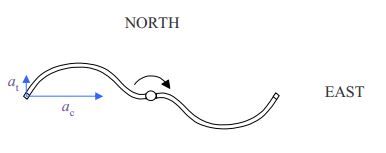
Now we just have to add the tangential acceleration and the centripetal acceleration vectorially to get the total acceleration. This is one of the easier kinds of vector addition problems since the vectors to be added are at right angles to each other.

From Pythagorean’s theorem we have
a=√a2c+a2t
a=√(260.6m/s2)2+(5.18m/s2)2
a=261m/s2
From the definition of the tangent of an angle as the opposite over the adjacent:
tanθ=atac
θ=tan−15.18m/s2260.6m/s2
θ=1.14∘
Thus,
a=261m/s2at 1.14∘ North of East
When the Angular Acceleration is not Constant
The angular position of a rotating body undergoing constant angular acceleration is given, as a function of time, by our first constant angular acceleration equation, equation ???:
θ=θ0+ω0t+12∝t2
If we take the 2nd derivative of this with respect to time, we get the constant ∝. (Recall that the first derivative yields the angular velocity ω and that ∝=dωdt. ) The expression on the right side of θ=θ0+ω0t+12∝t2 contains three terms: a constant, a term with t to the first power, and a term with t to the 2nd power. If you are given θ in terms of t, and it cannot be rearranged so that it appears as one of these terms or as a sum of two or all three such terms; then; ∝ is not a constant and you cannot use the constant angular acceleration equations. Indeed, if you are being asked to find the angular velocity at a particular instant in time, then you’ll want to take the derivative dθdt and evaluate the result at the given stopwatch reading. Alternatively, if you
are being asked to find the angular acceleration at a particular instant in time, then you’ll want to take the second derivative d2θdt2 and evaluate the result at the given stopwatch reading. Corresponding arguments can be made for the case of ω. If you are given ω as a function of t and the expression cannot be made to “look like” the constant angular acceleration equation ω=ω0+∝t then you are not dealing with a constant angular acceleration situation and you
should not use the constant angular acceleration equations.