
B30: The Electric Field Due to a Continuous Distribution of Charge on a Line
- Page ID
- 7888

\( \newcommand{\vecs}[1]{\overset { \scriptstyle \rightharpoonup} {\mathbf{#1}} } \)
\( \newcommand{\vecd}[1]{\overset{-\!-\!\rightharpoonup}{\vphantom{a}\smash {#1}}} \)
\( \newcommand{\dsum}{\displaystyle\sum\limits} \)
\( \newcommand{\dint}{\displaystyle\int\limits} \)
\( \newcommand{\dlim}{\displaystyle\lim\limits} \)
\( \newcommand{\id}{\mathrm{id}}\) \( \newcommand{\Span}{\mathrm{span}}\)
( \newcommand{\kernel}{\mathrm{null}\,}\) \( \newcommand{\range}{\mathrm{range}\,}\)
\( \newcommand{\RealPart}{\mathrm{Re}}\) \( \newcommand{\ImaginaryPart}{\mathrm{Im}}\)
\( \newcommand{\Argument}{\mathrm{Arg}}\) \( \newcommand{\norm}[1]{\| #1 \|}\)
\( \newcommand{\inner}[2]{\langle #1, #2 \rangle}\)
\( \newcommand{\Span}{\mathrm{span}}\)
\( \newcommand{\id}{\mathrm{id}}\)
\( \newcommand{\Span}{\mathrm{span}}\)
\( \newcommand{\kernel}{\mathrm{null}\,}\)
\( \newcommand{\range}{\mathrm{range}\,}\)
\( \newcommand{\RealPart}{\mathrm{Re}}\)
\( \newcommand{\ImaginaryPart}{\mathrm{Im}}\)
\( \newcommand{\Argument}{\mathrm{Arg}}\)
\( \newcommand{\norm}[1]{\| #1 \|}\)
\( \newcommand{\inner}[2]{\langle #1, #2 \rangle}\)
\( \newcommand{\Span}{\mathrm{span}}\) \( \newcommand{\AA}{\unicode[.8,0]{x212B}}\)
\( \newcommand{\vectorA}[1]{\vec{#1}} % arrow\)
\( \newcommand{\vectorAt}[1]{\vec{\text{#1}}} % arrow\)
\( \newcommand{\vectorB}[1]{\overset { \scriptstyle \rightharpoonup} {\mathbf{#1}} } \)
\( \newcommand{\vectorC}[1]{\textbf{#1}} \)
\( \newcommand{\vectorD}[1]{\overrightarrow{#1}} \)
\( \newcommand{\vectorDt}[1]{\overrightarrow{\text{#1}}} \)
\( \newcommand{\vectE}[1]{\overset{-\!-\!\rightharpoonup}{\vphantom{a}\smash{\mathbf {#1}}}} \)
\( \newcommand{\vecs}[1]{\overset { \scriptstyle \rightharpoonup} {\mathbf{#1}} } \)
\(\newcommand{\longvect}{\overrightarrow}\)
\( \newcommand{\vecd}[1]{\overset{-\!-\!\rightharpoonup}{\vphantom{a}\smash {#1}}} \)
\(\newcommand{\avec}{\mathbf a}\) \(\newcommand{\bvec}{\mathbf b}\) \(\newcommand{\cvec}{\mathbf c}\) \(\newcommand{\dvec}{\mathbf d}\) \(\newcommand{\dtil}{\widetilde{\mathbf d}}\) \(\newcommand{\evec}{\mathbf e}\) \(\newcommand{\fvec}{\mathbf f}\) \(\newcommand{\nvec}{\mathbf n}\) \(\newcommand{\pvec}{\mathbf p}\) \(\newcommand{\qvec}{\mathbf q}\) \(\newcommand{\svec}{\mathbf s}\) \(\newcommand{\tvec}{\mathbf t}\) \(\newcommand{\uvec}{\mathbf u}\) \(\newcommand{\vvec}{\mathbf v}\) \(\newcommand{\wvec}{\mathbf w}\) \(\newcommand{\xvec}{\mathbf x}\) \(\newcommand{\yvec}{\mathbf y}\) \(\newcommand{\zvec}{\mathbf z}\) \(\newcommand{\rvec}{\mathbf r}\) \(\newcommand{\mvec}{\mathbf m}\) \(\newcommand{\zerovec}{\mathbf 0}\) \(\newcommand{\onevec}{\mathbf 1}\) \(\newcommand{\real}{\mathbb R}\) \(\newcommand{\twovec}[2]{\left[\begin{array}{r}#1 \\ #2 \end{array}\right]}\) \(\newcommand{\ctwovec}[2]{\left[\begin{array}{c}#1 \\ #2 \end{array}\right]}\) \(\newcommand{\threevec}[3]{\left[\begin{array}{r}#1 \\ #2 \\ #3 \end{array}\right]}\) \(\newcommand{\cthreevec}[3]{\left[\begin{array}{c}#1 \\ #2 \\ #3 \end{array}\right]}\) \(\newcommand{\fourvec}[4]{\left[\begin{array}{r}#1 \\ #2 \\ #3 \\ #4 \end{array}\right]}\) \(\newcommand{\cfourvec}[4]{\left[\begin{array}{c}#1 \\ #2 \\ #3 \\ #4 \end{array}\right]}\) \(\newcommand{\fivevec}[5]{\left[\begin{array}{r}#1 \\ #2 \\ #3 \\ #4 \\ #5 \\ \end{array}\right]}\) \(\newcommand{\cfivevec}[5]{\left[\begin{array}{c}#1 \\ #2 \\ #3 \\ #4 \\ #5 \\ \end{array}\right]}\) \(\newcommand{\mattwo}[4]{\left[\begin{array}{rr}#1 \amp #2 \\ #3 \amp #4 \\ \end{array}\right]}\) \(\newcommand{\laspan}[1]{\text{Span}\{#1\}}\) \(\newcommand{\bcal}{\cal B}\) \(\newcommand{\ccal}{\cal C}\) \(\newcommand{\scal}{\cal S}\) \(\newcommand{\wcal}{\cal W}\) \(\newcommand{\ecal}{\cal E}\) \(\newcommand{\coords}[2]{\left\{#1\right\}_{#2}}\) \(\newcommand{\gray}[1]{\color{gray}{#1}}\) \(\newcommand{\lgray}[1]{\color{lightgray}{#1}}\) \(\newcommand{\rank}{\operatorname{rank}}\) \(\newcommand{\row}{\text{Row}}\) \(\newcommand{\col}{\text{Col}}\) \(\renewcommand{\row}{\text{Row}}\) \(\newcommand{\nul}{\text{Nul}}\) \(\newcommand{\var}{\text{Var}}\) \(\newcommand{\corr}{\text{corr}}\) \(\newcommand{\len}[1]{\left|#1\right|}\) \(\newcommand{\bbar}{\overline{\bvec}}\) \(\newcommand{\bhat}{\widehat{\bvec}}\) \(\newcommand{\bperp}{\bvec^\perp}\) \(\newcommand{\xhat}{\widehat{\xvec}}\) \(\newcommand{\vhat}{\widehat{\vvec}}\) \(\newcommand{\uhat}{\widehat{\uvec}}\) \(\newcommand{\what}{\widehat{\wvec}}\) \(\newcommand{\Sighat}{\widehat{\Sigma}}\) \(\newcommand{\lt}{<}\) \(\newcommand{\gt}{>}\) \(\newcommand{\amp}{&}\) \(\definecolor{fillinmathshade}{gray}{0.9}\)Every integral must include a differential (such as dx, dt, dq, etc.). An integral is an infinite sum of terms. The differential is necessary to make each term infinitesimal (vanishingly small). \(\int f(x)dx\) is okay, \(\int g(y)dy\) is okay, and \(\int h(t) dt\) is okay, but never write \(\int f(x)\), never write \(\int g(y)\) and never write \(\int h(t)\).
Here we revisit Coulomb’s Law for the Electric Field. Recall that Coulomb’s Law for the Electric Field gives an expression for the electric field, at an empty point in space, due to a charged particle. You have had practice at finding the electric field at an empty point in space due to a single charged particle and due to several charged particles. In the latter case, you simply calculated the contribution to the electric field at the one empty point in space due to each charged particle, and then added the individual contributions. You were careful to keep in mind that each contribution to the electric field at the empty point in space was an electric field vector, a vector rather than a scalar, hence the individual contributions had to be added like vectors.
A Review Problem for the Electric Field due to a Discrete Distribution of Charge
Let’s kick this chapter off by doing a review problem. The following example is one of the sort that you learned how to do when you first encountered Coulomb’s Law for the Electric Field. You are given a discrete distribution of source charges and asked to find the electric field (in the case at hand, just the \(x\) component of the electric field) at an empty point in space.
The example is presented on the next page. Here, a word about one piece of notation used in the solution. The symbol P is used to identify a point in space so that the writer can refer to that point, unambiguously, as “point \(P\).” The symbol \(P\) in this context does not stand for a variable or a constant. It is just an identification tag. It has no value. It cannot be assigned a value. It does not represent a distance. It just labels a point.
There are two charged particles on the x-axis of a Cartesian coordinate system, \(q_1\) at \(x=x_1\) and \(q_2\) at \(x=x_2\) where \(x_2>x_1\). Find the \(x\) component of the electric field, due to this pair of particles, valid for all points on the \(x\)-\(y\) plane for which \(x>x_2\). 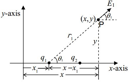
\(\vec{E_1}\) is the contribution to the electric field at point \(P\) (at x,y) due to charge \(q_1\). Charge \(q_2\) contributes to \(\vec{E_2}\) to the electric field at \(P\).
\(\vec{E}=\vec{E_1}+\vec{E_2}\)
\(E_x=E_{1x}+E_{2x}\)
First, let's get \(E_{1x}\):
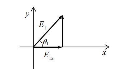
\(\frac{E_{1x}}{E_1}=\cos \theta_1\)
\(E_{1x}=E_1\cos\theta_1\)
Looking at the diagram at the top of this column, we see that Coulomb's Law for the Electric Field yields:
\(E_1=\frac{kq_1}{r_1^2}\)
\(E_{1x}=\frac{kq_1}{r_1^2}\cos\theta_1\)
Again, from that first diagram,
\(r_1=\sqrt{(x-x_1)^2+y^2}\)
and
\(\cos\theta_1=\frac{x-x_1}{r_1}=\frac{x-x_1}{\sqrt{(x-x_1)^2+y^2}}\)
Substitute both of these into \(E_{1x}=\frac{kq_1}{r_1^2}\cos\theta_1\) yields:
\(E_{1x}=\frac{kq_1}{(\sqrt{(x-x_1)^2+y^2})^2}\frac{x-x_1}{\sqrt{(x-x_1)^2+y^2}}\)
\(E_{1x}=\frac{kq_1(x-x_1)}{\Big[(x-x_1)^2+y^2 \Big] ^{\frac{3}{2}}}\)
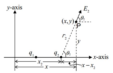
It is left as an exercise for the reader to show that:
\(E_{2x}=\frac{kq_2(x-x_2)}{\Big[(x-x_2)^2+y^2\Big]^{\frac{3}{2}}}\)
Since \(E_x=E_{1x}+E_{2x}\), we have:
\(E_x=\frac{kq_1(x-x_1)}{\Big[(x-x_2)^2+y^2\Big]^{\frac{3}{2}}}+\frac{kq_2(x-x_2)}{\Big[(x-x_2)^2+y^2\Big]^{\frac{3}{2}}}\)
\(\vec{E_1}\) is the contribution to the electric field at point \(P\) (at x,y) due to charge \(q_1\). Charge \(q_2\) contributes to \(\vec{E_2}\) to the electric field at \(P\).
\(\vec{E}=\vec{E_1}+\vec{E_2}\)
\(E_x=E_{1x}+E_{2x}\)
First, let's get \(E_{1x}\):
\(\frac{E_{1x}}{E_1}=\cos \theta_1\)
\(E_{1x}=E_1\cos\theta_1\)
Looking at the diagram at the top of this column, we see that Coulomb's Law for the Electric Field yields:
\(E_1=\frac{kq_1}{r_1^2}\)
\(E_{1x}=\frac{kq_1}{r_1^2}\cos\theta_1\)
Again, from that first diagram,
\(r_1=\sqrt{(x-x_1)^2+y^2}\)
and
\(\cos\theta_1=\frac{x-x_1}{r_1}=\frac{x-x_1}{\sqrt{(x-x_1)^2+y^2}}\)
Substitute both of these into \(E_{1x}=\frac{kq_1}{r_1^2}\cos\theta_1\) yields:
\(E_{1x}=\frac{kq_1}{(\sqrt{(x-x_1)^2+y^2})^2}\frac{x-x_1}{\sqrt{(x-x_1)^2+y^2}}\)
\(E_{1x}=\frac{kq_1(x-x_1)}{\Big[(x-x_1)^2+y^2 \Big] ^{\frac{3}{2}}}\)
It is left as an exercise for the reader to show that:
\(E_{2x}=\frac{kq_2(x-x_2)}{\Big[(x-x_2)^2+y^2\Big]^{\frac{3}{2}}}\)
Since \(E_x=E_{1x}+E_{2x}\), we have:
\(E_x=\frac{kq_1(x-x_1)}{\Big[(x-x_2)^2+y^2\Big]^{\frac{3}{2}}}+\frac{kq_2(x-x_2)}{\Big[(x-x_2)^2+y^2\Big]^{\frac{3}{2}}}\)
Linear Charge Density
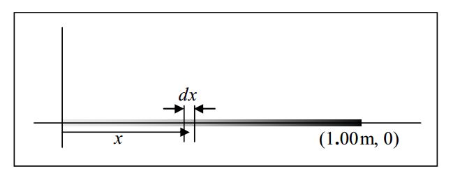
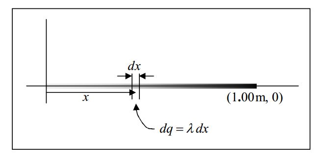
Okay, enough review, now lets consider the case in which we have a continuous distribution of charge along some line segment. In practice, we could be talking about a charged piece of string or thread, a charged thin rod, or even a charged piece of wire. First we need to discuss how one even specifies such a situation. We do so by stating what the linear charge density, the charge per-length, \(\lambda\) is. For now we’ll consider the meaning of \(\lambda\) for a few different situations (before we get to the heart of the matter, finding the electric field due to the linear charge distribution). Suppose for instance we have a one-meter string extending from the origin to \(x=1.00 m\) along the \(x\) axis, and that the linear charge density on that string is given by:
\[\lambda=1.56 \frac{\mu}{m^2}x. \nonumber \]
(Just under the equation, we have depicted the linear charge density graphically by drawing a line whose darkness represents the charge density.)
Note that if the value of \(x\) is expressed in meters, \(\lambda\) will have units of \(\frac{\mu C}{m}\), units of charge-per-length, as it must. Further note that for small values of \(x\), \(\lambda\) is small, and for larger values of \(x\), \(\lambda\) is larger. That means that the charge is more densely packed near the far (relative to the origin) end of the string. To further familiarize ourselves with what \(\lambda\) is, let’s calculate the total amount of charge on the string segment. What we’ll do is to get an expression for the amount of charge on any infinitesimal length \(dx\) of the string, and add up all such amounts of charge for all of the infinitesimal lengths making up the string segment.
The infinitesimal amount of charge \(dq\) on the infinitesimal length \(dx\) of the string is just the charge per length \(\lambda\) times the length \(dx\) of the infinitesimal string segment.
\[dq=\lambda dx \nonumber \]
Note that you can’t take the amount of charge on a finite length (such as \(15 cm\)) of the string to be \(\lambda\) times the length of the segment because \(\lambda\) varies over the length of the segment. In the case of an infinitesimal segment, every part of it is within an infinitesimal distance of the position specified by one and the same value of \(x\). The linear charge density doesn’t vary on an infinitesimal segment because \(x\) doesn’t—the segment is simply too short.
To get the total charge we just have to add up all the dq’s. Each dq is specified by its corresponding value of \(x\). To cover all the \(dq\)’s we have to take into account all the values of \(x\) from \(0\) to \(1.00\) m. Because each \(dq\) is the charge on an infinitesimal length of the line of charge, the sum is going to have an infinite number of terms. An infinite sum of infinitesimal pieces is an integral. When we integrate
\[dq=\lambda dx \nonumber \]
we get, on the left, the sum of all the infinitesimal pieces of charge making up the whole. By definition, the sum of all the infinitesimal amounts of charge is just the total charge \(Q\) (which by the way, is what we are solving for); we don’t need the tools of integral calculus to deal with the left side of the equation. Integrating both sides of the equation yields:
\[Q=\int_0^{1.00m} \lambda dx \nonumber \]
Using the given expression \(\lambda=1.56 \frac{\mu}{m^2}x\) we obtain
\[Q=\int_0^{1.00m} 2.56\frac{\mu C}{m^2}xdx=2.56\frac{\mu C}{m^2} \int_0^{1.00m}xdx=2.56 \frac{\mu C}{m^2} \frac{x^2}{2} \Big|_0^{1.00m}=2.56\frac{\mu C}{m^2} \Big[\frac{(1.00m)^2}{2}-\frac{(0)^2}{2}\Big]=1.28 \mu C \nonumber \]
A few more examples of distributions of charge follow:
For instance, consider charge distributed along the x axis, from \(x=0\) to \(x=L\) for the case in which the charge density is given by
\[\lambda=\lambda_{MAX} \sin(\pi \mbox{rad} x/L \nonumber \]
where \(\lambda_{MAX}\) is a constant having units of charge-per-length, rad stands for the units radians, \(x\) is the position variable, and \(L\) is the length of the charge distribution. Such a charge distribution has a maximum charge density equal to \(\lambda_{MAX}\) occurring in the middle of the line segment.
Another example would be a case in which charge is distributed on a line segment of length L extending along the y axis from \(y=a\) to \(y=a+L\) with a being a constant and the charge density given by
\[\lambda=\frac{38 \mu C \cdot m}{y^2} \nonumber \]
In this case the charge on the line is more densely packed in the region closer to the origin. (The smaller \(y\) is, the bigger the value of \(\lambda\), the charge-per-length.)
The simplest case is the one in which the charge is spread out uniformly over the line on which there is charge. In the case of a uniform linear charge distribution, the charge density is the same everywhere on the line of charge. In such a case, the linear charge density \(\lambda\) is simply a constant. Furthermore, in such a simple case, and only in such a simple case, the charge density \(\lambda\) is just the total amount of charge \(Q\) divided by the length \(L\) of the line along which that charge is uniformly distributed. For instance, suppose you are told that an amount of charge \(Q=2.45C\) is uniformly distributed along a thin rod of length \(L=0.840 m\). Then \(\lambda\) is given by:
\[\lambda=\frac{Q}{L} \nonumber \]
\[\lambda=\frac{2.45C}{0.840m} \nonumber \]
\[\lambda=2.92\frac{C}{m} \nonumber \]
The Electric Field Due to a Continuous Distribution of Charge along a Line
Okay, now we are ready to get down to the nitty-gritty. We are given a continuous distribution of charge along a straight line segment and asked to find the electric field at an empty point in space in the vicinity of the charge distribution. We will consider the case in which both the charge distribution and the empty point in space lie in the \(x\)-\(y\) plane. The values of the coordinates of the empty point in space are not necessarily specified. We can call them \(x\) and \(y\). In solving the problem for a single point in space with unspecified coordinates \((x,y)\), our final answer will have the symbols \(x\) and \(y\) in it, and our result will actually give the answer for an infinite set of points on the \(x\)-\(y\) plane.
The plan for solving such a problem is to find the electric field, due to an infinitesimal segment of the charge, at the one empty point in space. We do that for every infinitesimal segment of the charge, and then add up the results to get the total electric field.
Now once we chop up the charge distribution (in our mind, for calculational purposes) into infinitesimal (vanishingly small) pieces, we are going to wind up with an infinite number of pieces and hence an infinite sum when we go to add up the contributions to the electric field at the one single empty point in space due to all the infinitesimal segments of the linear charge distribution. That is to say, the result is going to be an integral.
An important consideration that we must address is the fact that the electric field, due to each element of charge, at the one empty point in space, is a vector. Hence, what we are talking about is an infinite sum of infinitesimal vectors. In general, the vectors being added are all in different directions from each other. (Can you think of a case so special that the infinite set of infinitesimal electric field vectors are all in the same direction as each other? Note that we are considering the general case, not such a special case.) We know better than to simply add the magnitudes of the vectors, infinite sum or not. Vectors that are not all in the same direction as each other, add like vectors, not like numbers. The thing is, however, the \(x\) components of all the infinitesimal electric field vectors at the one empty point in space do add like numbers. Likewise for the \(y\) components. Thus, if, for each infinitesimal element of the charge distribution, we find, not just the electric field at the empty point in space, but the \(x\) component of that electric field, then we can add up all the \(x\) components of the electric field at the empty point in space to get the \(x\) component of the electric field, due to the entire charge distribution, at the one empty point in space. The sum is still an infinite sum, but this time it is an infinite sum of scalars rather than vectors, and we have the tools for handling that. Of course, if we are asked for the total electric field, we have to repeat the entire procedure to get the \(y\) component of the electric field and then combine the two components of the electric field to get the total.
The easy way to do the last step is to use \(\hat{i},\hat{j},\hat{k}\) notation. That is, once we have \(E_x\) and \(E_y\), we can simply write:
\[\vec{E}=E_x \hat{i}+E_y \hat{j} \nonumber \]
Find the electric field valid for any point on the positive \(x\) axis due a \(36.0 cm\) long line of charge, lying on the \(y\) axis and centered on the origin, for which the charge density is given by \[\lambda=0.00120\frac{C}{m^2}y^2 \nonumber \]
As usual, we’ll start our solution with a diagram:
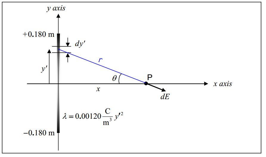
Note that we use (and strongly recommend that you use) primed quantities \((x′, y′)\) to specify a point on the charge distribution and unprimed quantities \((x, y)\) to specify the empty point in space at which we wish to know the electric field. Thus, in the diagram, the infinitesimal segment of the charge distribution is at \((0, y′)\) and point \(P\), the point at which we are finding the electric field, is at \((x,0)\). Also, our expression for the given linear charge density \(\lambda=0.00120\frac{C}{m^2}y^2\) expressed in terms of \(y′\) rather than y is:
\[\lambda=0.00120\frac{C}{m^2}y'^2 \nonumber \]
The plan here is to use Coulomb’s Law for the Electric Field to get the magnitude of the infinitesimal electric field vector \(\vec{dE}\) at point \(P\) due to the infinitesimal amount of charge \(dq\) in the infinitesimal segment of length \(dy′\).
\[dE=\frac{kdq}{r^2} \nonumber \]
The amount of charge \(dq\) in the infinitesimal segment \(dy′\) of the linear charge distribution is given by
\[dq=\lambda dy' \nonumber \]
From the diagram, it clear that we can use the Pythagorean theorem to express the distance \(r\) that point \(P\) is from the infinitesimal amount of charge \(dq\) under consideration as:
\[r=\sqrt{x^2+y'^2} \nonumber \]
Substituting this and \(dq=\lambda dy'\) into our equation for \(dE\) (\(dE=\frac{kdq}{r^2}\)) we obtain
\[dE=\frac{k\lambda dy'}{x^2+y'^2} \nonumber \]
Recall that our plan is to find \(E_x\), then \(E_y\) and then put them together using \(\vec{E}=E_x\hat{i}+E_y\hat{j}\). So for now, let’s get an expression for \(E_x\).
Based on the vector component diagram at right we have
\[dE_x=dE\cos\theta \nonumber \]
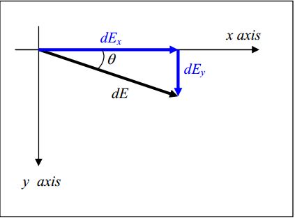
The \(\theta\) appearing in the diagram at right is the same \(\theta\) that appears in the diagram above. Based on the plane geometry evident in that diagram (above), we have:
\[\cos\theta=\frac{x}{r}=\frac{x}{\sqrt{x^2+y'^2}} \nonumber \]
Substituting both this expression for \(\cos \theta(\cos\theta=\frac{x}{\sqrt{x^2+y'^2}})\) and the expression we derived for \(dE\) above \((dE=\frac{k\lambda dy'}{(x^2+y'^2)^2})\) into the expression \(dE_x=dE\cos\theta\) from the vector component diagram yields:
\[(dE=\frac{k\lambda dy'}{(x^2+y'^2)^{\frac{3}{2}}}) \nonumber \]
Also, let’s go ahead and replace \(\lambda\) with the given expression \(\lambda=0.00120 \frac{C}{m^3}y'^2\):
\[dE_x=\Big(0.00120 \frac{C}{m^3} \Big) \frac{ky'^2x dy'}{(x^2+y'^2)^{\frac{3}{2}}} \nonumber \]
Now we have an expression for \(dE_x\) that includes only one quantity, namely \(y′\), that depends on which bit of the charge distribution is under consideration. Furthermore, although in the diagram

it appears that we picked out a particular infinitesimal line segment \(dy′\), in fact, the value of \(y′\) needed to establish its position is not specified. That is, we have an equation for \(dE_x\) that is good for any infinitesimal segment \(dy′\) of the given linear charge distribution. To identify a particular \(dy′\) we just have to specify the value of \(y′\). Thus to sum up all the \(dE_x’\)s we just have to add, to a running total, the \(dE_x\) for each of the possible values of \(y′\). Thus we need to integrate the expression for \(dE_x\) for all the values of \(y′\) from \(– 0.180 m\) to \(+0.180 m\).
\[\int dE_x=\int_{-0.180m}^{+0.180m} \Big( 0.00120 \frac{C}{m^3}\Big) \frac{ky'^2 xdy'}{(x^2+y'^2)^{\frac{3}{2}}} \nonumber \]
Copying that equation here:
\[\int dE_x=\int_{-0.180m}^{+0.180m} \Big( 0.00120 \frac{C}{m^3}\Big) \frac{ky'^2xdy'}{(x^2+y'^2)^{\frac{3}{2}}} \nonumber \]
we note that on the left is the infinite sum of all the contributions to the \(x\) component of the electric field due to all the infinitesimal elements of the line of charge. We don’t need any special mathematics techniques to evaluate that. The sum of all the parts is the whole. That is, on the left, we have \(E_x\).
The right side, we can evaluate. First, let’s factor out the constants:
\[E_x=\Big(0.00120 \frac{C}{m^3}\Big)kx \int_{-0.180m}^{+0.180m} \frac{y'^2dy'}{(x^2+y'^2)^{\frac{3}{2}}} \nonumber \]
The integral is given on your formula sheet. Carrying out the integration yields:
\[E_x=\Big(0.00120 \frac{C}{m^3} \Big)k x \Big[\frac{y'}{\sqrt{x^2+y'^2}}+ln(y'+\sqrt{x^2+y'^2}) \Big]_{-0.180m}^{+0.180m} \nonumber \]
\[E_x=\Big(.00120\frac{C}{m^3}\Big) kx\cdot\Big\{\Big( \Big[ \frac{+.018m}{\sqrt{x^2+(+.180m)^2}}+ln\Big( +.018m+\sqrt{x^2+(+.018m)^2}\Big) \Big]- \nonumber \]
\[\Big[ \frac{-.180m}{\sqrt{x^2+(-.180)^2}}+ln(-.180m+\sqrt{x^2+(-.180m)^2})\Big]\Big\} \nonumber \]
\[E_x=\Big(.00120\frac{C}{m^3}\Big) kx\cdot \Big[\frac{.360m}{\sqrt{x^2+(.180m)^2}}+\ln \frac{\sqrt{x^2+(.180m)^2}+.180m}{\sqrt{x^2+(.180m)^2}-.180m}\Big] \nonumber \]
Substituting the value of the Coulomb constant k from the formula sheet we obtain
\[E_x=\Big(.00120\frac{C}{m^3}\Big)8.99\times 10^9 \frac{N\cdot m^2}{C^2}x\cdot\Big[ \frac{.360m}{\sqrt{x^2+(.180m)^2}}+\ln \frac{\sqrt{x^2+(.180m)^2}+.180m}{\sqrt{x^2+(.180m)^2}-.180m}\Big] \nonumber \]
Finally we have
\[E_x=1.08\times10^7\frac{N}{C\cdot m}\cdot \Big[\frac{.360m}{\sqrt{x^2+(.180m)^2}}+\ln \frac{\sqrt{x^2+(.180m)^2}+.180m}{\sqrt{x^2+(.180m)^2}-.180m}\Big] \nonumber \]
It is interesting to note that while the position variable x (which specifies the location of the empty point in space at which the electric field is being calculated) is a constant for purposes of integration (the location of point \(P\) does not change as we include the contribution to the electric field at point \(P\) of each of the infinitesimal segments making up the charge distribution), an actual value \(x\) was never specified. Thus our final result
\[E_x=1.08\times 10^7 \frac{N}{C\cdot m} x \cdot \Big[\frac{.360m}{\sqrt{x^2+(.180m)^2}}+\ln\frac{\sqrt{x^2+(.180m)^2}+.180m}{\sqrt{x^2+(.180m)^2}-.180m}\Big ] \nonumber \]
for \(E_x\) is a function of the position variable \(x\).
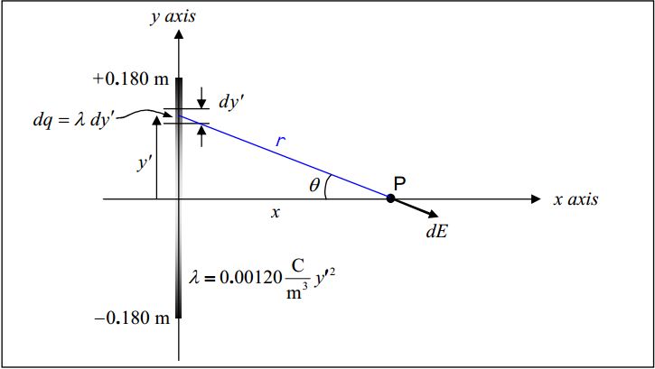
Getting the y-component of the electric field can be done with a lot less work than it took to get \(E_x\) if we take advantage of the symmetry of the charge distribution with respect to the \(x\) axis. Recall that the charge density \(\lambda\), for the case at hand, is given by:
\[\lambda=0.00120\frac{C}{m^3} y'^2 \nonumber \]
Because \(\lambda\) is proportional to \(y'^2\), the value of \(\lambda\) is the same at the negative of a specified \(y'\) value as it is at the \(y'\) value itself. More specifically, the amount of charge in each of the two samesize infinitesimal elements \(dy′\) of the charge distribution depicted in the following diagram:
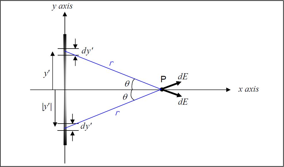
is one and the same value because one element is the same distance below the \(x\) axis as the other is above it. This position circumstance also makes the distance \(r\) that each element is from point P the same as that of the other, and, it makes the two angles (each of which is labeled \(\theta\) in the diagram) have one and the same value. Thus the two \(\vec{dE}\) vectors have one and the same magnitude. As a result of the latter two facts (same angle, same magnitude of \(\vec{dE}\)), the \(y\) components of the two \(\vec{dE}\) vectors cancel each other out. As can be seen in the diagram under consideration:
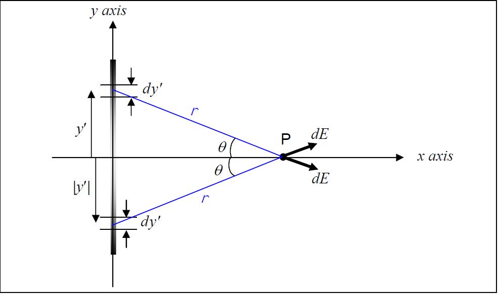
one is in the \(+y\) direction and the other in the \(–y\) direction. The \(y\) components are “equal and opposite.”) In fact, for each and every charge distribution element \(dy′\) that is above the \(x\) axis and is thus creating a downward contribution to the \(y\) component of the electric field at point \(P\), there is an element \(dy′\) that is the same distance below the x axis that is creating an upward contribution to the \(y\) component of the electric field at point \(P\), canceling the \(y\) component of the
former. Thus the net sum of all the electric field \(y\) components (since they cancel pair-wise) is zero. That is to say that due to the symmetry of the charge distribution with respect to the \(x\) axis, \(E_y=0\). Thus,
\[\vec{E}=E_x \hat{i} \nonumber \]
Using the expression for \(E_x\) that we found above, we have, for our final answer:
\[\vec{E}=1.08\times 10^7\frac{N}{C\cdot m} x\Big[\frac{.360m}{\sqrt{x^2+(.180m)^2}}+\ln\frac{\sqrt{x^2+(.180m)^2}+.180m}{\sqrt{x^2+(.180m)^2}-.180m}\Big] \hat{i} \nonumber \]
former. Thus the net sum of all the electric field \(y\) components (since they cancel pair-wise) is zero. That is to say that due to the symmetry of the charge distribution with respect to the \(x\) axis, \(E_y=0\). Thus,