
B35: Gauss’s Law for the Magnetic Field and Ampere’s Law Revisited


- Last updated
- Jan 16, 2023
- Save as PDF

( \newcommand{\kernel}{\mathrm{null}\,}\)
Gauss’s Law for the Magnetic Field
Remember Gauss’s Law for the electric field? It’s the one that, in conceptual terms, states that the number of electric field lines poking outward through a closed surface is proportional to the amount of electric charge inside the closed surface. In equation form, we wrote it as:
∮→E⋅→dA=Qenclosedϵo
We called the quantity on the left the electric flux ΦE=∮→E⋅→dA.
Well, there is a Gauss’s Law for the magnetic field as well. In one sense, it is quite similar because it involves a quantity called the magnetic flux which is expressed mathematically as ΦB=∮→B⋅→dA and represents the number of magnetic field lines poking outward through a closed surface. The big difference stems from the fact that there is no such thing as “magnetic charge.” In other words, there is no such thing as a magnetic monopole. In Gauss’s Law for the electric field we have electric charge (divided by ϵo) on the right. In Gauss’s Law for the magnetic field, we have 0 on the right:
∮→B⋅→dA=0
As far as calculating the magnetic field, this equation is of limited usefulness. But, in conjunction with Ampere’s Law in integral form (see below), it can come in handy for calculating the magnetic field in cases involving a lot of symmetry. Also, it can be used as a check for cases in which the magnetic field has been determined by some other means.
Ampere’s Law
We’ve talked about Ampere’s Law quite a bit already. It’s the one that says a current causes a magnetic field. Note that this one says nothing about anything changing. It’s just a cause and effect relation. The integral form of Ampere’s Law is both broad and specific. It reads:
∮→B⋅→dℓ=μoITHROUGH
where:
∘ the circle on the integral sign, and, →dℓ, the differential length, together, tell you that the integral (the infinite sum) is around an imaginary closed loop.
→B is the magnetic field,
→dℓ is an infinitesimal path element of the closed loop,
μo is a universal constant called the magnetic permeability of free space, and
ITHROUGH is the current passing through the region enclosed by the loop.
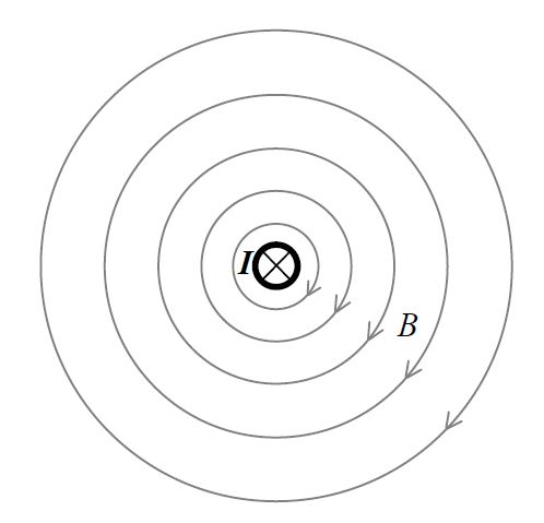
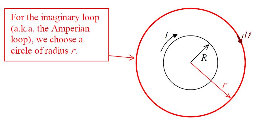
What Ampere’s Law in integral form says is that, if you sum up the magnetic-field along-a-pathsegment times the length of the path segment for all the path segments making up an imaginary closed loop, you get the current through the region enclosed by the loop, times a universal constant. The integral ∮→B⋅→dℓ on whatever closed path upon which it is carried out, is called the circulation of the magnetic field on that closed path. So, another way of stating the integral form of Ampere’s Law is to say that the circulation of the magnetic field on any closed path is directly proportional to the current through the region enclosed by the path. Here’s the picture:

In the picture, I show everything except for the magnetic field. The idea is that, for each infinitesimal segment →dℓ of the imaginary loop, you dot the magnetic field →B, at the position of the segment, into →dℓ. Add up all such dot products. The total is equal to μ0 times the current I through the loop.
So, what’s it good for? Ampere’s Law in integral form is of limited use to us. It can be used as a great check for a case in which one has calculated the magnetic field due to some set of current-carrying conductors some other way (e.g. using the Biot-Savart Law, to be introduced in the next chapter). Also, in cases involving a high degree of symmetry, we can use it to calculate the magnetic field due to some current.
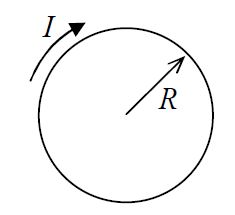
For example, we can use Ampere’s Law to get a mathematical expression for the magnitude of the magnetic field due to an infinitely-long straight wire. I’m going to incorporate our understanding that, for a segment of wire with a current in it, the current creates a magnetic field which forms loops about the wire in accord with the right-hand rule for something curly something straight. In other words, we already know that for a long straight wire carrying current directly away from you, the magnetic field extends in loops about the wire, which, from your vantage point, are clockwise.
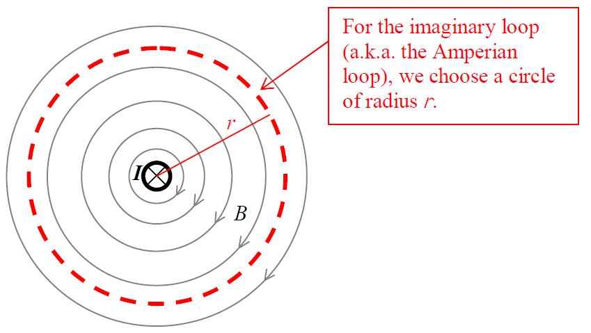
From symmetry, we can argue that the magnitude of the magnetic field is the same for a given point as it is at any other point that is the same distance from the wire as that given point. In implementing Ampere’s Law, it is incumbent upon us to choose an imaginary loop, called an Amperian Loop in this context, that allows us to get some useful information from Ampere’s Law. In this case, a circle whose plane is perpendicular to the straight wire and whose center lies on the straight wire is a smart choice.
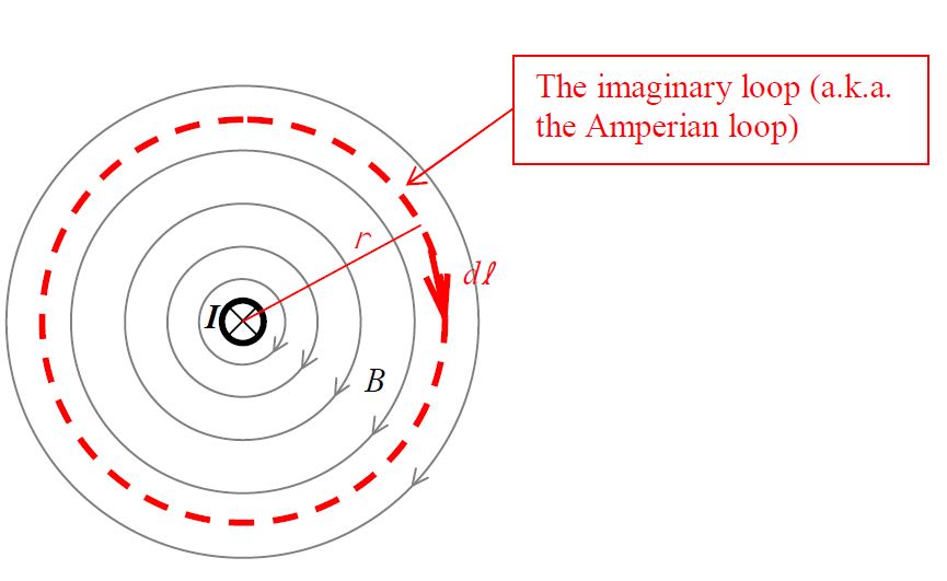
At this point I want to share with you some directional information about the integral form of Ampere’s Law. Regarding the →dℓ: each →dℓ vector can, from a given point of view, be characterized as representing either a clockwise step along the path or a counterclockwise step along the path. And, if one is clockwise, they all have to be clockwise. If one is counterclockwise, they all have to be counterclockwise. Thus, in carrying out the integral around the closed loop, the traversal of the loop is either clockwise or counterclockwise from a specified viewpoint. Now, here’s the critical direction information: Current that passes through the loop in that direction which relates to the sense (clockwise or counterclockwise) of loop traversal in accord with the right-hand rule for something curly something straight (with the loop being the something curly and the current being the something straight) is considered positive. So, for the case at hand, if I choose a clockwise loop traversal, as viewed from the vantage point that makes things look like:
then, the current I is considered positive. If you curl the fingers around the loop in the clockwise direction, your thumb points away from you. This means that current, through the loop that is directed away from you is positive. That is just the kind of current we have in the case at hand. So, when we substitute the I for the case at hand into the generic equation (Ampere’s Law),
∮→B⋅→dℓ=μoITHROUGH
for the current μoITHROUGH it goes in with a "+" sign.
∮→B⋅→dℓ=μoI
Now, with the loop I chose, every →dℓ is exactly parallel to the magnetic field →B at the location of the →dℓ, so, →B⋅→dℓ is simply B dℓ. That is, with our choice of Amperian loop, Ampere’s Law simplifies to:
∮Bdℓ=μoI
Furthermore, from symmetry, with our choice of Amperian loop, the magnitude of the magnetic field B has one and the same value at every point on the loop. That means we can factor the magnetic field magnitude B out of the integral. This yields:
B∮dℓ=μoI
Okay, now we are on easy street. The ∮dℓ is just the sum of all the dℓ's making up our imaginary loop (a circle) of radius r. Hey, that’s just the circumference of the circle 2πr. So, Ampere’s Law becomes:
B(2πr)=μoI
which means
B=μoI2πr
This is our end result. The magnitude of the magnetic field due to a long straight wire is directly proportional to the current in the wire and inversely proportional to the distance from the wire.
A Long Straight Solenoid
A solenoid is a coil of wire in the form of a cylindrical shell. The idealized solenoid that we consider here is infinitely long but, it has a fixed finite radius R and a constant finite current I.
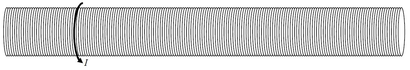
It is also characterized by its number-of-turns-per-length, n, where each “turn” (a.k.a. winding) is one circular current loop. In fact, we further idealize our solenoid by thinking of it as an infinite set of circular current loops. An actual solenoid approaches this idealized solenoid, but, in one turn (in the view above), the end of the turn is displaced left or right from the start of the turn by an amount equal to the diameter of the wire. As a result, in an actual solenoid, we have (in the view above) some left-to-right or right-to-left (depending on which way the wire wraps around) current. We neglect this current and consider the current to just go “round and round.”
Our goal here is to find the magnetic field due to an ideal infinitely-long solenoid that has a number-of-turns-per-length n, has a radius R, and carries a current I.
We start by looking at the solenoid in cross section. Relative to the view above, we’ll imagine looking at the solenoid from the left end. From that point of view, the cross section is a circle with clockwise current:
Let’s try an Amperian loop in the shape of a circle, whose plane is perpendicular to the axis of symmetry of the solenoid, a circle that is centered on the axis of symmetry of the solenoid.
From symmetry, we can argue that if the magnetic field has a component parallel to the depicted dℓ, then it must have the exact same component for every dℓ on the closed path. But this would make the circulation ∮→B⋅→dℓ non-zero in contradiction to the fact that no current passes through the region enclosed by the loop. This is true for any value of r. So, the magnetic field can have no component tangent to the circle whose plane is perpendicular to the axis of symmetry of the solenoid, a circle that is centered on the axis of symmetry of the solenoid.
Now suppose the magnetic field has a radial component. By symmetry it would have to be everywhere directed radially outward from the axis of symmetry of the solenoid, or everywhere radially inward. In either case, we could construct an imaginary cylindrical shell whose axis of symmetry coincides with that of the solenoid. The net magnetic flux through such a Gaussian surface would be non-zero in violation of Gauss’s Law for the magnetic field. Hence the solenoid can have no radial magnetic field component.
The only kind of field that we haven’t ruled out is one that is everywhere parallel to the axis of symmetry of the solenoid. Let’s see if such a field would lead to any contradictions.
Here we view the solenoid in cross-section from the side. At the top of the coil, we see the current directed toward us, and, at the bottom, away. The possible longitudinal (parallel to the axis of symmetry of the solenoid) magnetic field is included in the diagram.
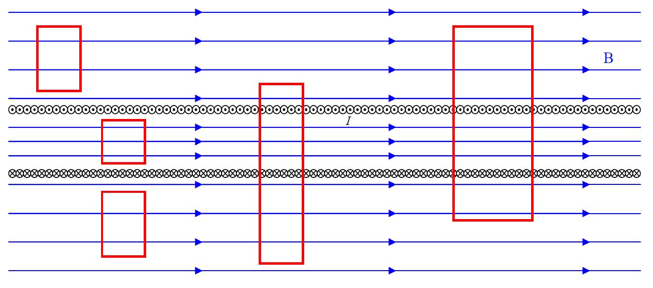
The rectangles in the diagram represent Amperian loops. The net current through any of the loops, in either direction (away from you or toward you) is zero. As such, the circulation ∮→B⋅→dℓ is zero. Since the magnetic field on the right and left of any one of the loops is perpendicular to the right and left sides of any one of the loops, it makes no contribution to the circulation there. By symmetry, the magnetic field at one position on the top of a loop is the same as it is at any other point on the top of the same loop. Hence, if we traverse any one of the loops counterclockwise (from our viewpoint) the contribution to the circulation is −BTOPL where L is the length of the top and bottom segments of whichever loop you choose to focus your attention on. The "-" comes from the fact that I have (arbitrarily) chosen to traverse the loop counterclockwise, and, in doing so, every →dℓ in the top segment is in the opposite direction to the direction of the magnetic field at the top of the loop. The contribution to the circulation by the bottom segment of the same loop is +BBOTTOML. What we have so far is:
∮→B⋅→dℓ=μoITHROUGH
∮→B⋅→dℓ=0
(where the net current through any one of the loops depicted is zero by inspection.)
0+−BTOPL+0+BBOTTOML=0
(with the two zeros on the left side of the equation being from the right and left sides of the loop where the magnetic field is perpendicular to the loop.)
Solving for BBOTTOM we find that, for every loop in the diagram (and the infinite number of loops enclosing a net current of zero just like them):
BBOTTOM=BTOP
What this means is that the magnetic field at all points outside the solenoid has one and the same magnitude. The same can be said about all points inside the solenoid, but, the inside the solenoid value may be different from the outside value. In fact, let’s consider a loop through which the net current is not zero:
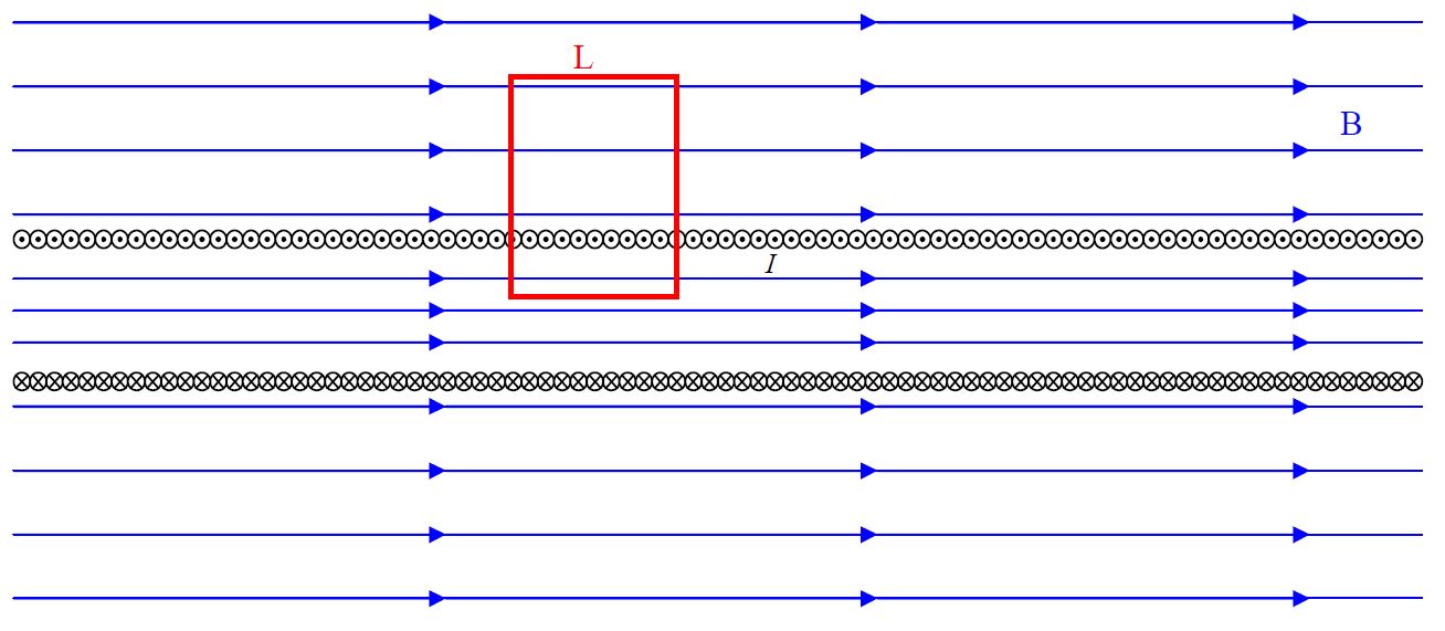
Again, I choose to go counterclockwise around the loop (from our viewpoint). As such, by the right-hand rule for something curly something straight, current directed toward us through the loop is positive. Recalling that the number-of-turns-per-length-of-the-solenoid is n, we have, for the loop depicted above,
∮→B⋅→dℓ=μoITHROUGH
0+−BTOPL+0+BBOTTOML=μonLI
BBOTTOM=BTOP+μonI
The bottom of the loop is inside the solenoid and we have established that the magnitude of the magnetic field inside the solenoid has one and the same magnitude at all points inside the solenoid. I’m going to call that BINSIDE, meaning that BBOTTOM=BINSIDE. Similarly, we have found that the magnitude of the magnetic field has one and the same (other) value at all points outside the solenoid. Let’s call that BOUTSIDE, meaning that BTOP=BOUTSIDE. Thus:
BINSIDE=BOUTSIDE+μonI
This is as far as I can get with Gauss’s Law for the magnetic field, symmetry, and Ampere’s Law alone. From there I turn to experimental results with long finite solenoids. Experimentally, we find that the magnetic field outside the solenoid is vanishingly small, and that there is an appreciable magnetic field inside the solenoid. Setting
BOUTSIDE=0
we find that the magnetic field inside a long straight solenoid is:
BINSIDE=μonI