9.6: Sound Waves

So far, we mostly considered transversal waves, which include waves in strings and waves on the surface of a pond, and are easily visualized. Longitudinal waves, on the other hand, are somewhat harder to draw, but easily heard - as sound is the prime example of a longitudinal wave. Other examples include (some forms of) seismic waves and ultrasound. Many people simply lump all of these together, and use the terms ‘sound waves’ and ‘longitudinal waves’ as synonyms

Figure \(\PageIndex{1}\): Snapshots of the wave patterns for the first three modes of a standing wave in (a) a string with two clamped ends, (b) a string with one clamped end, or a tube with one closed and one open end, and (c) a tube with two open ends. In each case, the plot shows the amplitude of the standing wave, as a fraction of the amplitude of the traveling wave. At nodes, the amplitude of the standing wave vanishes: destructive interference causes these points to always stand still. At antinodes, the amplitude of the standing wave is maximal, and equals that of the traveling wave. Note that (a) and (b) will occur for transversal waves, whereas (b) and (c) will occur for sound waves. For cases (a) and (c) allowed wavelengths are \(\lambda = \frac{2L}{n}\), whereas for case (b), allowed wavelengths are \(\lambda = \frac{4L}{(2n −1)}\).

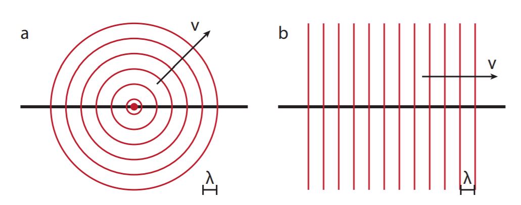
We already touched upon the speed of sound waves in Section 9.2 (Equation 9.2.10). This speed indicates how fast the wavefronts of a sound wave travel; a wavefront is defined as the surface (in three dimensions) where all points have the same phase.¹ To visualize a sound wave we draw a succession of wavefronts one wavelength (or one period) apart. Simple examples include a point source (generating spherical wavefronts) and a planar wave, in which all wave fronts are parallel planes (Figure \(\PageIndex{2}\)). The (local) direction of propagation of the wave is the direction perpendicular to the wavefronts, sometimes depicted by a ray.

Figure \(\PageIndex{2}\): Snapshots of the wavefronts (points with equal phase) of a longitudinal wave for (a) a point source (with spherical wavefronts) and (b) a planar wave (where all wavefronts are parallel planes). Successive wavefronts are separated by one wavelength.

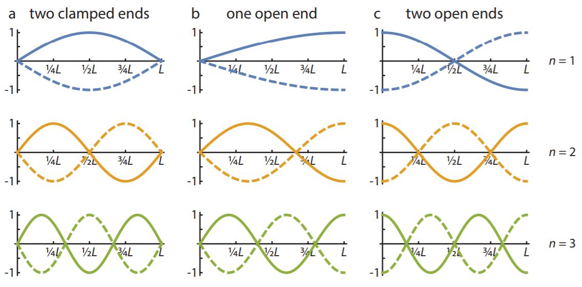
Like transversal waves, longitudinal waves exhibit interference, both with other waves they encounter, and by their own reflections. There can therefore be traveling and standing sound waves. Unlike transversal waves on strings however, longitudinal sound waves are typically created in tubes that are open on either one or both ends. A closed end represents a fixed point, just like the fixed end of a string does, resulting in a stringent boundary condition: the interference between the incoming and outgoing wave must be such that the net displacement at the closed end is zero. An open end corresponds to a transversal wave in a string that is not clamped. As the string in that case is free to move, its maximum displacement will equal the amplitude of the wave. In other words, while a closed end corresponds to a node, the open end corresponds to an antinode. For a string (or pipe) with one clamped / closed and one open end, the wavelength of the lowest order mode (known as the fundamental mode or first harmonic) therefore equals four times the length \(L\) of the string / pipe. The next mode (second harmonic) will have a wavelength of \(4L/3\), and so on (Figure \(\PageIndex{2b}\)), resulting in \(\lambda = 4L/(2n − 1)\) for the \(n\)th mode. For a tube with two open ends, the fundamental mode is the inverse of that of a string with two clamped ends - so two antinodes at the ends, and a node in the middle (Figure 9.6.1c). Like for a clamped string, the allowed wavelengths are therefore \(\lambda = 2L/n\).

¹ A wavefront corresponding to the maximum extension \(u\) is sometimes called a wavecrest.