8.2: Projectile Motion

Projectile motion is basically just free fall, only with the understanding that the object we are tracking was “projected,” or “shot,” with some initial velocity (as opposed to just dropped from rest). Unlike in the previous cases of free fall that we have studied so far, we will now assume that the initial velocity has a horizontal component, as a result of which, instead of just going straight up and/or down, the object will describe (ignoring air resistance, as usual) a parabola in a vertical plane.

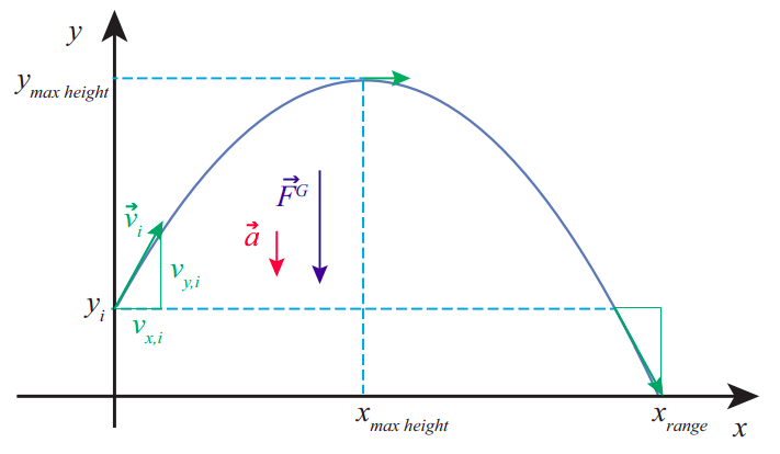
The plane in question is determined by the initial velocity (more precisely, the horizontal component of the initial velocity) and gravity. A generic trajectory is shown in Figure \(\PageIndex{1}\), showing the force and acceleration vectors (constant throughout) and the velocity vector at various points along the path.

Figure \(\PageIndex{1}\): A typical projectile trajectory. The velocity vector (in green) is shown at the initial time, the point of maximum height, and the point where the projectile is back to its initial height.

Conceptually, the problem turns out to be extremely simple if we apply the basic principle introduced in Section 8.1. The force is vertical throughout; so, after the throw, there is no horizontal acceleration, and the vertical acceleration is just \(−g\), just as it always was in our earlier, onedimensional free-fall problems:

\begin{align}
&a_{x}=\frac{F_{x}}{m}=0 \nonumber \\
&a_{y}=\frac{F_{y}}{m}=-g \label{eq:8.4}.
\end{align}

The overall motion, then, is a combination of motion with constant velocity horizontally, and motion with constant acceleration vertically, and we can write down the corresponding equations of motion immediately:

\begin{align}
v_{x} &=v_{x, i} \nonumber \\
v_{y} &=v_{y, i}-g t \nonumber \\
x &=x_{i}+v_{x, i} t \nonumber \\
y &=y_{i}+v_{y, i} t-\frac{1}{2} g t^{2} \label{eq:8.5}
\end{align}

where (\(x_i, y_i\)) are the coordinates of the launching point (there is usually no reason to make \(x_i\) anything other than zero, so we will do that below), and (\(v_{x,i}, v_{y,i}\)) the initial components of the velocity vector.

By eliminating \(t\) in between the last two Eqs. (\ref{eq:8.5}), we get the equation of the trajectory in the \(x\)-\(y\) plane:

\[ y=y_{i}+\frac{v_{y, i}}{v_{x, i}} x-\frac{g}{2 v_{x, i}^{2}} x^{2} \label{eq:8.6} \]

which, as indicated earlier, and as shown in Figure \(\PageIndex{1}\), is indeed the equation of a parabola.

The apex of the parabola (highest point in the trajectory) is at \(x_{max \: height} = v_{x,i}v_{y,i}/g\). We can get this result from calculus, or from a comparison of Equation (\ref{eq:8.6}) with the canonical form of a parabola, or we can use some physics: the maximum height is reached, as usual, when the vertical velocity becomes momentarily zero, so solving the \(v_y\) equation (\ref{eq:8.5}) for \(t_{max \: height}\) and substituting in the \(x\) equation, we get

\begin{align}
&t_{\text {max height }}=\frac{v_{y, i}}{g} \nonumber \\
&x_{\text {max height }}=\frac{v_{x, i} v_{y, i}}{g}\nonumber \\
&y_{\text {max height }}=y_{i}+\frac{v_{y, i}^{2}}{2 g} \label{eq:8.7}.
\end{align}

The last of these equations should look familiar. It is, indeed a variation on our old friend \(v^2_f − v^2_i = −2g\Delta y\), only now instead of the full velocity \(\vec v\) we have to use only the vertical velocity component \(v_y\). Just like for one-dimensional motion, this result follows again from conservation of energy: throughout the flight, we must have \(K + U^G\) = constant, only now there is a component to the kinetic energy—the part associated with the horizontal motion—which remains constant on its own. In general, the kinetic energy of a particle will be \(\frac{1}{2}m|\vec v|^2\), where \(|\vec v|\) is the magnitude of the velocity vector—that is to say, the speed. In two dimensions, this gives

\[ K=\frac{1}{2} m v_{x}^{2}+\frac{1}{2} m v_{y}^{2} \label{eq:8.8} .\]

For projectile motion, however, \(v_x\) does not change, so any change in \(K\) will affect only the second term in Equation (\ref{eq:8.8}). Conservation of energy between any two instants \(i\) and \(f\) gives

\[ K+U^{G}=\frac{1}{2} m v_{x, i}^{2}+\frac{1}{2} m v_{y, i}^{2}+m g y_{i}=\frac{1}{2} m v_{x, i}^{2}+\frac{1}{2} m v_{y, f}^{2}+m g y_{f} \label{eq:8.9} .\]

The \(\frac{1}{2}mv^2_{x,i}\) term cancels, and therefore

\[ v_{y, f}^{2}-v_{y, i}^{2}=-2 g\left(y_{f}-y_{i}\right) \label{eq:8.10} .\]

Another quantity of interest is the projectile’s range, or maximum horizontal distance traveled. We can calculate it from Eqs. (\ref{eq:8.5}), by setting \(y\) equal to the final height, then solving for \(t\) (which generally requires solving a quadratic equation), and then substituting the result in the equation for \(x\). In the simple case when the final height is the same as the initial height, we can avoid the need for calculating altogether, and just reason, from the fact that the trajectory is symmetric, that the total horizontal distance traveled will be twice the distance to the point where the maximum height is reached, that is, \(x_{range} = 2x_{max \: height}\):

\[ x_{\text {range }} = \frac{2 v_{x, i} v_{y, i}}{g} \quad \text { (only if }\left.y_{f}=y_{i}\right) \label{eq:8.11} .\]

As you can see, all these equations depend on the initial values of the components of the velocity vector \(\vec v_i\). If \(\vec v_i\) makes an angle \(\theta\) with the horizontal, and we simplify the notation by calling its magnitude \(v_i\), then we can write

\begin{align}
&v_{x, i}=v_{i} \cos \theta \nonumber \\
&v_{y, i}=v_{i} \sin \theta \label{eq:8.12}
\end{align}

In terms of \(v_i\) and \(\theta\), the range equation (\ref{eq:8.11}) becomes

\[ x_{\text {range }}=\frac{v_{i}^{2} \sin (2 \theta)}{g} \quad \text { (only if } y_{f}=y_{i}) \label{eq:8.13} \]

since \(2 \sin \theta \cos \theta = \sin(2\theta)\). This tells us that for any given launch speed, the maximum range is achieved when the launch angle \(\theta = 45^{\circ}\) (always assuming the final height is the same as the initial height).

In real life, of course, there will always be air resistance, and all these results will be modified somewhat. Mathematically, things become a lot more complicated: the drag force depends on the speed, which involves both components of the velocity, so the horizontal and vertical motions are no longer decoupled: not only is there now an \(F_x\), but its value at any given time depends both on \(v_x\) and \(v_y\). Physically, you may think of the drag force as doing negative work on the projectile, and hence removing kinetic energy from it. Less kinetic energy means, basically, that it will not travel quite as far either vertically or horizontally. Surprisingly, the optimum launch angle remains pretty close to 45\(^{\circ}\), at least if the simulations at this link are accurate:

https://phet.colorado.edu/en/simulation/projectile-motion