

11: HR Diagram and Stellar Evolution
- Page ID
- 163003

\( \newcommand{\vecs}[1]{\overset { \scriptstyle \rightharpoonup} {\mathbf{#1}} } \)
\( \newcommand{\vecd}[1]{\overset{-\!-\!\rightharpoonup}{\vphantom{a}\smash {#1}}} \)
\( \newcommand{\dsum}{\displaystyle\sum\limits} \)
\( \newcommand{\dint}{\displaystyle\int\limits} \)
\( \newcommand{\dlim}{\displaystyle\lim\limits} \)
\( \newcommand{\id}{\mathrm{id}}\) \( \newcommand{\Span}{\mathrm{span}}\)
( \newcommand{\kernel}{\mathrm{null}\,}\) \( \newcommand{\range}{\mathrm{range}\,}\)
\( \newcommand{\RealPart}{\mathrm{Re}}\) \( \newcommand{\ImaginaryPart}{\mathrm{Im}}\)
\( \newcommand{\Argument}{\mathrm{Arg}}\) \( \newcommand{\norm}[1]{\| #1 \|}\)
\( \newcommand{\inner}[2]{\langle #1, #2 \rangle}\)
\( \newcommand{\Span}{\mathrm{span}}\)
\( \newcommand{\id}{\mathrm{id}}\)
\( \newcommand{\Span}{\mathrm{span}}\)
\( \newcommand{\kernel}{\mathrm{null}\,}\)
\( \newcommand{\range}{\mathrm{range}\,}\)
\( \newcommand{\RealPart}{\mathrm{Re}}\)
\( \newcommand{\ImaginaryPart}{\mathrm{Im}}\)
\( \newcommand{\Argument}{\mathrm{Arg}}\)
\( \newcommand{\norm}[1]{\| #1 \|}\)
\( \newcommand{\inner}[2]{\langle #1, #2 \rangle}\)
\( \newcommand{\Span}{\mathrm{span}}\) \( \newcommand{\AA}{\unicode[.8,0]{x212B}}\)
\( \newcommand{\vectorA}[1]{\vec{#1}} % arrow\)
\( \newcommand{\vectorAt}[1]{\vec{\text{#1}}} % arrow\)
\( \newcommand{\vectorB}[1]{\overset { \scriptstyle \rightharpoonup} {\mathbf{#1}} } \)
\( \newcommand{\vectorC}[1]{\textbf{#1}} \)
\( \newcommand{\vectorD}[1]{\overrightarrow{#1}} \)
\( \newcommand{\vectorDt}[1]{\overrightarrow{\text{#1}}} \)
\( \newcommand{\vectE}[1]{\overset{-\!-\!\rightharpoonup}{\vphantom{a}\smash{\mathbf {#1}}}} \)
\( \newcommand{\vecs}[1]{\overset { \scriptstyle \rightharpoonup} {\mathbf{#1}} } \)
\(\newcommand{\longvect}{\overrightarrow}\)
\( \newcommand{\vecd}[1]{\overset{-\!-\!\rightharpoonup}{\vphantom{a}\smash {#1}}} \)
\(\newcommand{\ket}[1]{\left| #1 \right>}\)
\(\newcommand{\bra}[1]{\left< #1 \right|}\)
\(\newcommand{\braket}[2]{\left< #1 \vphantom{#2} \right| \left. #2 \vphantom{#1} \right>}\)
\(\newcommand{\braopket}[3]{\left< #1 \vphantom{#2}\vphantom{#3} \right| #2 \vphantom{#1}\vphantom{#3} \left| #3 \vphantom{#1}\vphantom{#2} \right>}\)
\(\newcommand{\qmvec}[1]{\mathbf{\vec{#1}}}\)
\(\newcommand{\op}[1]{\hat{\mathbf{#1}}}\)
\(\newcommand{\expect}[1]{\langle #1 \rangle}\)
\(\newcommand{\dfn}[1]{\emph{\textbf{#1}}}\)
Lab Overview
Lab Goals
As a result of this lab, you should be able to:
- Describe and compare the phases of stellar evolution for low, medium, and high mass stars
- Identify trends on an HR diagram relating to luminosity, temperature/color, and stellar radius
- Identify a directional relationship between stellar mass and main-sequence life-time.
Equipment and Setup
This lab requires the following equipment on each table.
- Computers with internet for simulation
Submission Instructions
Submit a brief lab report that includes the following sections:
Results
HR Diagram sketches with annotations and values plotted
Discussion
Write clear paragraphs that answer the discussion questions throughout the lab. When relevant, be sure to cite evidence from the results section and explain how that evidence supports your claims.
Part 1: HR Diagram and Stella Origin Point
Simulation Setup
- Open the simulation at https://astro.unl.edu/naap/hr/animations/hrExplorer.html
- The red line represents the Main Sequence and can be thought of as the starting point of a star’s life
Collecting Data
- Click on different parts of the red line to see a visual of the different stars
- Draw circles on your results HR Diagram that show:
- Size
- Color
- Click around near where you drew your circles and write the value for Radius next to them. A radius of 1 means the radius of our sun.
- Nearest Stars
- Select Nearest Stars and put dots on your diagram to show the general star locations plotted (you do not need to copy every dot exactly)
- Click around on some of them to look for common trends about color and size. Add labels to your diagram based on the trends
- Brightest Stars
- Select Brightest Stars and put dots on your diagram to show the general star locations plotted (you do not need to copy every dot exactly)
- Click around on some of them to look for common trends about color and size. Add labels to your diagram based on the trends
- Add radius values next to some of the points to help show trends.
- Isoradius Lines
- Make sure the show isoradius lines box is checked
- Sketch these lines with their radius values on your diagram
- Draw arrows between lines in the direction that radius increases.
Discussion Questions:
- Where on an HR Diagram are the hottest (most blue) and coldest (most red) stars?
- How does the size of a star change based on location on an HR diagram?
Part 2: One Stellar-mass Star
Simulation Setup
- Open the simulation at https://www.starinabox.net/ and select Advanced
- Set the Mass to 1 (should be the default)
- Play the simulation (you can adjust speed if you want)
- Replay the simulation as needed at different speeds. You can also click on the diagram to show that point in time (best when simulation is paused)
Collecting Data
- Sketch the “path” of the star on from the simulation
- Highlight parts of the path different colors to match the color of the star
- Add labels on the path to identify if radius is increasing or decreasing
- Add the stage labels on the different parts of the stellar evolution path
- Place dots at transitions from one stage to the next and put the age of the star next to those dots.
Identify Trends
Try to identify trends on the diagram (locations or directions) for the following:
- Star Color
- Star Size
- Where the most time is spent (you need to use the years because the animation speed is not constant).
You can add information about these trends on the diagram or on the lines below the diagram
Discussion Questions:
- What stage is a star in for most of its lifetime? How does the mass of the star affect the time spent in this stage?
- When a star gets bigger does it get more red or more blue? Identify patterns in changing size to color and temperature.
Part 3: Lower and Higher Mass Stars
Simulation Setup
- Set the Mass to each of the following values: 0.5, 8, 30
- Follow the same set of instructions as for the one solar-mass star.
- You can explore other mass stars if you finish early
Discussion Questions:
- What are the different possible end states of stars? What determines which end state a star will reach?
Templates
HR Diagram
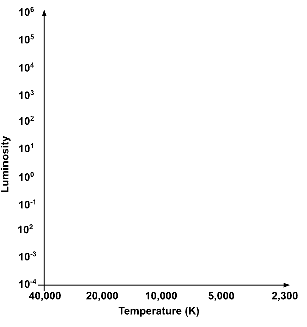
Stellar Evolution
