7.5: Applications of Magnetic Forces and Fields

Learning Objectives

By the end of this section, you will be able to:

• Explain how a mass spectrometer works to separate charges
• Explain how a cyclotron works

Being able to manipulate and sort charged particles allows deeper experimentation to understand what matter is made of. We first look at a mass spectrometer to see how we can separate ions by their charge-to-mass ratio. Then we discuss cyclotrons as a method to accelerate charges to very high energies.

Mass Spectrometer

The mass spectrometer is a device that separates ions according to their charge-to-mass ratios. One particular version, the Bainbridge mass spectrometer, is illustrated in Figure \(\PageIndex{1}\). Ions produced at a source are first sent through a velocity selector, where the magnetic force is equally balanced with the electric force. These ions all emerge with the same speed \(v = E/B\) since any ion with a different velocity is deflected preferentially by either the electric or magnetic force, and ultimately blocked from the next stage. They then enter a uniform magnetic field \(B_0\) where they travel in a circular path whose radius R is given by Equation 11.4.2, \(r = \frac{mv}{qB}\). The radius is measured by a particle detector located as shown in the figure.

Figure \(\PageIndex{1}\): A schematic of the Bainbridge mass spectrometer, showing charged particles leaving a source, followed by a velocity selector where the electric and magnetic forces are balanced, followed by a region of uniform magnetic field where the particle is ultimately detected.

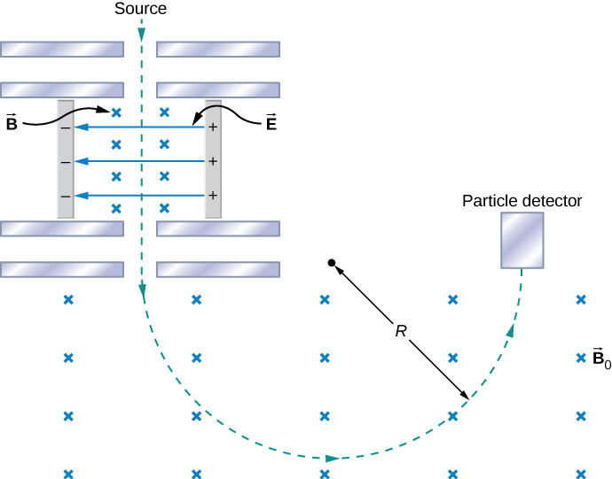
The relationship between the charge-to-mass ratio q/m and the radius R is determined by combining Equation 11.4.2 and Equation 11.7.2:

\[\frac{q}{m} = \frac{E}{BB_0R}.\]

Since most ions are singly charged \((q = 1.6 \times 10^{-10}C)\), measured values of R can be used with this equation to determine the mass of ions. With modern instruments, masses can be determined to one part in \(10^8\).

An interesting use of a spectrometer is as part of a system for detecting very small leaks in a research apparatus. In low-temperature physics laboratories, a device known as a dilution refrigerator uses a mixture of He-3, He-4, and other cryogens to reach temperatures well below 1 K. The performance of the refrigerator is severely hampered if even a minute leak between its various components occurs. Consequently, before it is cooled down to the desired temperature, the refrigerator is subjected to a leak test. A small quantity of gaseous helium is injected into one of its compartments, while an adjacent, but supposedly isolated, compartment is connected to a high-vacuum pump to which a mass spectrometer is attached. A heated filament ionizes any helium atoms evacuated by the pump. The detection of these ions by the spectrometer then indicates a leak between the two compartments of the dilution refrigerator.

In conjunction with gas chromatography, mass spectrometers are used widely to identify unknown substances. While the gas chromatography portion breaks down the substance, the mass spectrometer separates the resulting ionized molecules. This technique is used with fire debris to ascertain the cause, in law enforcement to identify illegal drugs, in security to identify explosives, and in many medicinal applications.

Cyclotron

The cyclotron was developed by E.O. Lawrence to accelerate charged particles (usually protons, deuterons, or alpha-particles) to large kinetic energies. These particles are then used for nuclear-collision experiments to produce radioactive isotopes. A cyclotron is illustrated in Figure \(\PageIndex{2}\). The particles move between two flat, semi-cylindrical metallic containers D1 and D2, called dees. The dees are enclosed in a larger metal container, and the apparatus is placed between the poles of an electromagnet that provides a uniform magnetic field. Air is removed from the large container so that the particles neither lose energy nor are deflected because of collisions with air molecules. The dees are connected to a high-frequency voltage source that provides an alternating electric field in the small region between them. Because the dees are made of metal, their interiors are shielded from the electric field.

Figure \(\PageIndex{2}\): The inside of a cyclotron. A uniform magnetic field is applied as circulating protons travel through the dees, gaining energy as they traverse through the gap between the dees.

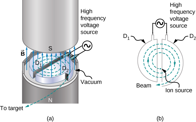
Suppose a positively charged particle is injected into the gap between the dees when D2 is at a positive potential relative to D1. The particle is then accelerated across the gap and enters D1 after gaining kinetic energy qV, where V is the average potential difference the particle experiences between the dees. When the particle is inside D1, only the uniform magnetic field \(\vec{B}\) of the electromagnet acts on it, so the particle moves in a circle of radius

\[r = \frac{mv}{qB} \label{11.32}\]

with a period of

\[T = \frac{2\pi m}{qB}. \label{11.33}\]

The period of the alternating voltage course is set at T, so while the particle is inside D1, moving along its semicircular orbit in a time T/2, the polarity of the dees is reversed. When the particle reenters the gap, D1 is positive with respect to D2, and the particle is again accelerated across the gap, thereby gaining a kinetic energy qV. The particle then enters D2, circulates in a slightly larger circle, and emerges from D2 after spending a time T/2 in this dee. This process repeats until the orbit of the particle reaches the boundary of the dees. At that point, the particle (actually, a beam of particles) is extracted from the cyclotron and used for some experimental purpose.

The operation of the cyclotron depends on the fact that, in a uniform magnetic field, a particle’s orbital period is independent of its radius and its kinetic energy. Consequently, the period of the alternating voltage source need only be set at the one value given by Equation \ref{11.33}. With that setting, the electric field accelerates particles every time they are between the dees.

If the maximum orbital radius in the cyclotron is R, then from Equation \ref{11.32}, the maximum speed of a circulating particle of mass m and charge q is

\[v_{max} = \frac{qBR}{m}.\]

Thus, its kinetic energy when ejected from the cyclotron is

\[\frac{1}{2}mv_{max}^2 = \frac{q^2B^2R^2}{2m}.\]

The maximum kinetic energy attainable with this type of cyclotron is approximately 30 MeV. Above this energy, relativistic effects become important, which causes the orbital period to increase with the radius. Up to energies of several hundred MeV, the relativistic effects can be compensated for by making the magnetic field gradually increase with the radius of the orbit. However, for higher energies, much more elaborate methods must be used to accelerate particles.

Particles are accelerated to very high energies with either linear accelerators or synchrotrons. The linear accelerator accelerates particles continuously with the electric field of an electromagnetic wave that travels down a long evacuated tube. The Stanford Linear Accelerator (SLAC) is about 3.3 km long and accelerates electrons and positrons (positively charged electrons) to energies of 50 GeV. The synchrotron is constructed so that its bending magnetic field increases with particle speed in such a way that the particles stay in an orbit of fixed radius. The world’s highest-energy synchrotron is located at CERN, which is on the Swiss-French border near Geneva. CERN has been of recent interest with the verified discovery of the Higgs Boson (see Particle Physics and Cosmology). This synchrotron can accelerate beams of approximately \(10^{13}\) protons to energies of about \(10^3\) GeV.

Example \(\PageIndex{1}\): Accelerating Alpha-Particles in a Cyclotron

A cyclotron used to accelerate alpha-particles \((m = 6.64 \times 10^{-27} kg, \, q = 3.2 \times 10^{-19}C)\) has a radius of 0.50 m and a magnetic field of 1.8 T. (a) What is the period of revolution of the alpha-particles? (b) What is their maximum kinetic energy?

Strategy

1. The period of revolution is approximately the distance traveled in a circle divided by the speed. Identifying that the magnetic force applied is the centripetal force, we can derive the period formula.
2. The kinetic energy can be found from the maximum speed of the beam, corresponding to the maximum radius within the cyclotron.

Solution

1. By identifying the mass, charge, and magnetic field in the problem, we can calculate the period: \[T = \frac{2\pi m}{qB} = \frac{2\pi (6.64 \times 10^{-27} kg)}{(3.2 \times 10^{-19}C)(1.8 T)} = 7.3 \times 10^{-8} s.\]
2. By identifying the charge, magnetic field, radius of path, and the mass, we can calculate the maximum kinetic energy: \[\frac{1}{2} mv_{max}^2 = \frac{q^2B^2R^2}{2m} = \frac{(3.2 \times 10^{-19}C)^2(1.8 T)^2(0.50 m)^2}{2(6.65 \times 10^{-27}kg)} = 6.2 \times 10^{-12}J = 39 \, MeV.\]

Exercise \(\PageIndex{1}\)

A cyclotron is to be designed to accelerate protons to kinetic energies of 20 MeV using a magnetic field of 2.0 T. What is the required radius of the cyclotron?

Solution

0.32 m

Mass Spectrometry

The curved paths followed by charged particles in magnetic fields can be put to use. A charged particle moving perpendicular to a magnetic field travels in a circular path having a radius \(r\).

\[r = \frac{mv}{qB}\label{22.12.1}\]

It was noted that this relationship could be used to measure the mass of charged particles such as ions. A mass spectrometer is a device that measures such masses. Most mass spectrometers use magnetic fields for this purpose, although some of them have extremely sophisticated designs. Since there are five variables in the relationship, there are many possibilities. However, if \(v\), \(q\), and \(B\) can be fixed, then the radius of the path \(r\) is simply proportional to the mass \(m\) of the charged particle. Let us examine one such mass spectrometer that has a relatively simple design (Figure \(\PageIndex{1}\)). The process begins with an ion source, a device like an electron gun. The ion source gives ions their charge, accelerates them to some velocity \(v\), and directs a beam of them into the next stage of the spectrometer. This next region is a velocity selector that only allows particles with a particular value of \(v\) to get through.

Figure \(\PageIndex{1}\): This mass spectrometer uses a velocity selector to fix \(v\) so that the radius of the path is proportional to mass.

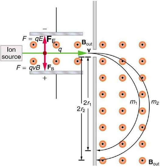
The velocity selector has both an electric field and a magnetic field, perpendicular to one another, producing forces in opposite directions on the ions. Only those ions for which the forces balance travel in a straight line into the next region. If the forces balance, then the electric force \(F = qE\) equals the magnetic force \(F = qvB\), so that \(qE = qvB\). Noting that \(q\) cancels, we see that

\[v = \frac{E}{B}\label{22.12.2}\]

is the velocity particles must have to make it through the velocity selector, and further, that \(v\) can be selected by varying \(E\) and \(B\). In the final region, there is only a uniform magnetic field, and so the charged particles move in circular arcs with radii proportional to particle mass. The paths also depend on charge \(q\), but since \(q\) is in multiples of electron charges, it is easy to determine and to discriminate between ions in different charge states.

Mass spectrometry today is used extensively in chemistry and biology laboratories to identify chemical and biological substances according to their mass-to-charge ratios. In medicine, mass spectrometers are used to measure the concentration of isotopes used as tracers. Usually, biological molecules such as proteins are very large, so they are broken down into smaller fragments before analyzing. Recently, large virus particles have been analyzed as a whole on mass spectrometers. Sometimes a gas chromatograph or high-performance liquid chromatograph provides an initial separation of the large molecules, which are then input into the mass spectrometer.

Cathode Ray Tubes—CRTs—and the Like

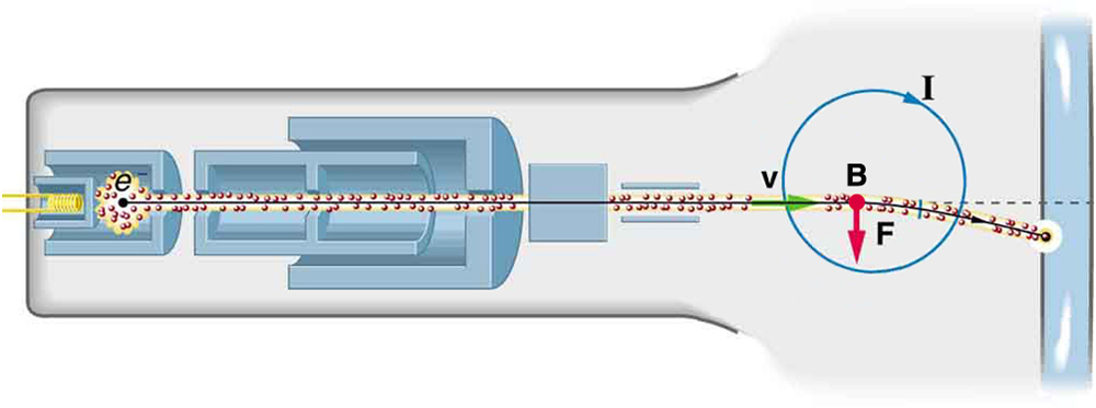
What do non-flat-screen TVs, old computer monitors, x-ray machines, and the 2-mile-long Stanford Linear Accelerator have in common? All of them accelerate electrons, making them different versions of the electron gun. Many of these devices use magnetic fields to steer the accelerated electrons. Figure \(\PageIndex{2}\) shows the construction of the type of cathode ray tube (CRT) found in some TVs, oscilloscopes, and old computer monitors. Two pairs of coils are used to steer the electrons, one vertically and the other horizontally, to their desired destination.

Figure \(\PageIndex{2}\): The cathode ray tube (CRT) is so named because rays of electrons originate at the cathode in the electron gun. Magnetic coils are used to steer the beam in many CRTs. In this case, the beam is moved down. Another pair of horizontal coils would steer the beam horizontally.

Magnetic Resonance Imaging

Magnetic resonance imaging (MRI) is one of the most useful and rapidly growing medical imaging tools. It non-invasively produces two-dimensional and three-dimensional images of the body that provide important medical information with none of the hazards of x-rays. MRI is based on an effect called nuclear magnetic resonance (NMR) in which an externally applied magnetic field interacts with the nuclei of certain atoms, particularly those of hydrogen (protons). These nuclei possess their own small magnetic fields, similar to those of electrons and the current loops discussed earlier in this chapter.

When placed in an external magnetic field, such nuclei experience a torque that pushes or aligns the nuclei into one of two new energy states—depending on the orientation of its spin (analogous to the N pole and S pole in a bar magnet). Transitions from the lower to higher energy state can be achieved by using an external radio frequency signal to “flip” the orientation of the small magnets. (This is actually a quantum mechanical process. The direction of the nuclear magnetic field is quantized as is energy in the radio waves. We will return to these topics in later chapters.) The specific frequency of the radio waves that are absorbed and reemitted depends sensitively on the type of nucleus, the chemical environment, and the external magnetic field strength. Therefore, this is a resonance phenomenon in which nuclei in a magnetic field act like resonators (analogous to those discussed in the treatment of sound in "Oscillatory Motion and Waves") that absorb and reemit only certain frequencies. Hence, the phenomenon is named nuclear magnetic resonance (NMR).

NMR has been used for more than 50 years as an analytical tool. It was formulated in 1946 by F. Bloch and E. Purcell, with the 1952 Nobel Prize in Physics going to them for their work. Over the past two decades, NMR has been developed to produce detailed images in a process now called magnetic resonance imaging (MRI), a name coined to avoid the use of the word “nuclear” and the concomitant implication that nuclear radiation is involved. (It is not.) The 2003 Nobel Prize in Medicine went to P. Lauterbur and P. Mansfield for their work with MRI applications.

The largest part of the MRI unit is a superconducting magnet that creates a magnetic field, typically between 1 and 2 T in strength, over a relatively large volume. MRI images can be both highly detailed and informative about structures and organ functions. It is helpful that normal and non-normal tissues respond differently for slight changes in the magnetic field. In most medical images, the protons that are hydrogen nuclei are imaged. (About 2/3 of the atoms in the body are hydrogen.) Their location and density give a variety of medically useful information, such as organ function, the condition of tissue (as in the brain), and the shape of structures, such as vertebral disks and knee-joint surfaces. MRI can also be used to follow the movement of certain ions across membranes, yielding information on active transport, osmosis, dialysis, and other phenomena. With excellent spatial resolution, MRI can provide information about tumors, strokes, shoulder injuries, infections, etc.

An image requires position information as well as the density of a nuclear type (usually protons). By varying the magnetic field slightly over the volume to be imaged, the resonant frequency of the protons is made to vary with position. Broadcast radio frequencies are swept over an appropriate range and nuclei absorb and reemit them only if the nuclei are in a magnetic field with the correct strength. The imaging receiver gathers information through the body almost point by point, building up a tissue map. The reception of reemitted radio waves as a function of frequency thus gives position information. These “slices” or cross sections through the body are only several mm thick. The intensity of the reemitted radio waves is proportional to the concentration of the nuclear type being flipped, as well as information on the chemical environment in that area of the body. Various techniques are available for enhancing contrast in images and for obtaining more information. Scans called T1, T2, or proton density scans rely on different relaxation mechanisms of nuclei. Relaxation refers to the time it takes for the protons to return to equilibrium after the external field is turned off. This time depends upon tissue type and status (such as inflammation).

While MRI images are superior to x rays for certain types of tissue and have none of the hazards of x rays, they do not completely supplant x-ray images. MRI is less effective than x rays for detecting breaks in bone, for example, and in imaging breast tissue, so the two diagnostic tools complement each other. MRI images are also expensive compared to simple x-ray images and tend to be used most often where they supply information not readily obtained from x rays. Another disadvantage of MRI is that the patient is totally enclosed with detectors close to the body for about 30 minutes or more, leading to claustrophobia. It is also difficult for the obese patient to be in the magnet tunnel. New “open-MRI” machines are now available in which the magnet does not completely surround the patient.

Over the last decade, the development of much faster scans, called “functional MRI” (fMRI), has allowed us to map the functioning of various regions in the brain responsible for thought and motor control. This technique measures the change in blood flow for activities (thought, experiences, action) in the brain. The nerve cells increase their consumption of oxygen when active. Blood hemoglobin releases oxygen to active nerve cells and has somewhat different magnetic properties when oxygenated than when deoxygenated. With MRI, we can measure this and detect a blood oxygen-dependent signal. Most of the brain scans today use fMRI.

Other Medical Uses of Magnetic Fields

Currents in nerve cells and the heart create magnetic fields like any other currents. These can be measured but with some difficulty since their strengths are about \(10^{-6}\) to \(10^{-8}\) less than the Earth’s magnetic field. Recording of the heart’s magnetic field as it beats is called a magnetocardiogram (MCG), while measurements of the brain's magnetic field is called a magnetoencephalogram (MEG). Both give information that differs from that obtained by measuring the electric fields of these organs (ECGs and EEGs), but they are not yet of sufficient importance to make these difficult measurements common.

In both of these techniques, the sensors do not touch the body. MCG can be used in fetal studies, and is probably more sensitive than echocardiography. MCG also looks at the heart’s electrical activity whose voltage output is too small to be recorded by surface electrodes as in EKG. It has the potential of being a rapid scan for early diagnosis of cardiac ischemia (obstruction of blood flow to the heart) or problems with the fetus.

MEG can be used to identify abnormal electrical discharges in the brain that produce weak magnetic signals. Therefore, it looks at brain activity, not just brain structure. It has been used for studies of Alzheimer’s disease and epilepsy. Advances in instrumentation to measure very small magnetic fields have allowed these two techniques to be used more in recent years. What is used is a sensor called a SQUID, for superconducting quantum interference device. This operates at liquid helium temperatures and can measure magnetic fields thousands of times smaller than the Earth’s.

Finally, there is a burgeoning market for magnetic cures in which magnets are applied in a variety of ways to the body, from magnetic bracelets to magnetic mattresses. The best that can be said for such practices is that they are apparently harmless, unless the magnets get close to the patient’s computer or magnetic storage disks. Claims are made for a broad spectrum of benefits from cleansing the blood to giving the patient more energy, but clinical studies have not verified these claims, nor is there an identifiable mechanism by which such benefits might occur.

Contributors and Attributions

Samuel J. Ling (Truman State University), Jeff Sanny (Loyola Marymount University), and Bill Moebs with many contributing authors. This work is licensed by OpenStax University Physics under a Creative Commons Attribution License (by 4.0).