6.4: Drawing Free-Body Diagrams

Learning Objectives

• Explain the rules for drawing a free-body diagram
• Construct free-body diagrams for different situations

The first step in describing and analyzing most phenomena in physics involves the careful drawing of a free-body diagram. Free-body diagrams have been used in examples throughout this chapter. Remember that a free-body diagram must only include the external forces acting on the body of interest. Once we have drawn an accurate free-body diagram, we can apply Newton’s first law if the body is in equilibrium (balanced forces; that is, \(F_{net} = 0\)) or Newton’s second law if the body is accelerating (unbalanced force; that is, \(F_{net} \neq 0\)).

Problem-Solving Strategy: Constructing Free-Body Diagrams

Observe the following rules when constructing a free-body diagram:

1. Draw the object under consideration; it does not have to be artistic. At first, you may want to draw a circle around the object of interest to be sure you focus on labeling the forces acting on the object. If you are treating the object as a particle (no size or shape and no rotation), represent the object as a point. We often place this point at the origin of an xy-coordinate system.
2. Include all forces that act on the object, representing these forces as vectors. Consider the types of forces described in Common Forces—normal force, friction, tension, and spring force—as well as weight and applied force. Do not include the net force on the object. With the exception of gravity, all of the forces we have discussed require direct contact with the object. However, forces that the object exerts on its environment must not be included. We never include both forces of an action-reaction pair.
3. Convert the free-body diagram into a more detailed diagram showing the x- and y-components of a given force (this is often helpful when solving a problem using Newton’s first or second law). In this case, place a squiggly line through the original vector to show that it is no longer in play—it has been replaced by its x- and y-components.
4. If there are two or more objects, or bodies, in the problem, draw a separate free-body diagram for each object.

Note: If there is acceleration, we do not directly include it in the free-body diagram; however, it may help to indicate acceleration outside the free-body diagram. You can label it in a different color to indicate that it is separate from the free-body diagram.

Let’s apply the problem-solving strategy in drawing a free-body diagram for a sled. In Figure \(\PageIndex{1a}\), a sled is pulled by force \(\vec{P}\) at an angle of 30°. In part (b), we show a free-body diagram for this situation, as described by steps 1 and 2 of the problem-solving strategy. In part (c), we show all forces in terms of their x- and y-components, in keeping with step 3.

Figure \(\PageIndex{1}\): (a) A moving sled is shown as (b) a free-body diagram and (c) a free-body diagram with force components.

 

Example \(\PageIndex{1}\)

Figure \(\PageIndex{1}\): A block on a horizontal table.

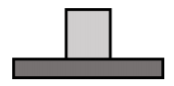
A block of mass \(m\) is at rest on a horizontal table, as shown in Figure \(\PageIndex{1}\). What forces are exerted on the block?

Solution

The forces on the block are illustrated in Figure \(\PageIndex{2}\) and are:

1. \(\vec F_g\), its weight.
2. \(\vec N\), a normal force exerted by the plane. The normal force is perpendicular to the interface between the table and the block. It points upwards in “reaction” to the downwards force that the block exerts onto the table. The downwards force from the block onto the table is not shown, since that force is not exerted on the block but on the table.

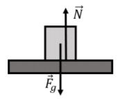
Figure \(\PageIndex{2}\): Forces on a block on a horizontal table.

Example \(\PageIndex{2}\)

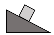
A block of mass \(m\) is at rest on a inclined surface, as shown in Figure 5.4.3. What forces are exerted on the block?

Figure \(\PageIndex{3}\): A block on an inclined surface.

Solution

The forces on the block are illustrated in Figure \(\PageIndex{4}\) and are:

1. \(\vec F_g\), its weight.
2. \(\vec N\), a normal force exerted by the inclined plane.
3. \(\vec f_s\), a force of static friction exerted by the inclined plane. Without this force, the block would slide down. The force is in the direction opposite of impeding motion and is parallel to the interface (and perpendicular to the normal force).

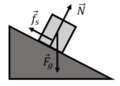
Figure \(\PageIndex{4}\): Forces on block on an inclined surface.

Example \(\PageIndex{3}\)

Figure \(\PageIndex{5}\): A block resting on a wedge-shaped block.

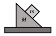
A block of mass \(m\) is at rest on a wedge-shaped block of mass \(M\) itself at rest on a horizontal table, as shown in Figure \(\PageIndex{5}\). What forces are exerted on each of the two blocks?

Solution

Since it will be too messy to draw all of the forces on the same diagram, we have drawn each block separately in Figure \(\PageIndex{5}\). Usually, when multiple blocks are stacked on each other, it is easiest to start with the forces on the top block. In this case, the top block is in the same condition as the block from Example 5.4.2. The forces exerted on the top block are:

1. \(\vec F_g^m\), its weight.
2. \(\vec N^m\), a normal force from the wedge-shaped block.
3. \(\vec f_s^m\), a force of static friction exerted by the wedge-shaped block.

The forces exerted on the wedge-shaped block are:

1. \(\vec F_g^M\), its weight.
2. \(\vec N^M\), a normal force exerted by the small block. Note that this force is equal in magnitude and opposite in direction to \(\vec N^m\) (the two forces, \(\vec N^m\) and \(\vec N^M\), which are on different objects, are an action/reaction pair of forces).
3. \(\vec f_s^M\), a force of friction exerted by the small block (again, this forms an action/reaction pair of forces with \(\vec f_s^m\)).
4. \(N_2^M\), a normal force exerted by the table.

The forces for both blocks are shown in Figure \(\PageIndex{6}\).

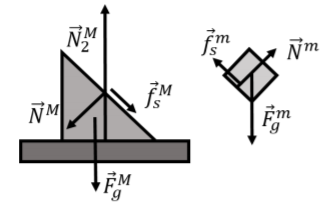
Figure \(\PageIndex{6}\): Forces on the block and the wedge-shaped block.

Example \(\PageIndex{4}\): Two Blocks on an Inclined Plane

Construct the free-body diagram for object A and object B in Figure \(\PageIndex{1}\).

Strategy

We follow the four steps listed in the problem-solving strategy.

Solution

We start by creating a diagram for the first object of interest. In Figure \(\PageIndex{2a}\), object A is isolated (circled) and represented by a dot.

Figure \(\PageIndex{2}\): (a) The free-body diagram for isolated object A. (b) The free-body diagram for isolated object B. Comparing the two drawings, we see that friction acts in the opposite direction in the two figures. Because object A experiences a force that tends to pull it to the right, friction must act to the left. Because object B experiences a component of its weight that pulls it to the left, down the incline, the friction force must oppose it and act up the ramp. Friction always acts opposite the intended direction of motion.

We now include any force that acts on the body. Here, no applied force is present. The weight of the object acts as a force pointing vertically downward, and the presence of the cord indicates a force of tension pointing away from the object. Object A has one interface and hence experiences a normal force, directed away from the interface. The source of this force is object B, and this normal force is labeled accordingly. Since object B has a tendency to slide down, object A has a tendency to slide up with respect to the interface, so the friction f_BA is directed downward parallel to the inclined plane.

As noted in step 4 of the problem-solving strategy, we then construct the free-body diagram in Figure 5.32(b) using the same approach. Object B experiences two normal forces and two friction forces due to the presence of two contact surfaces. The interface with the inclined plane exerts external forces of N_B and f_B, and the interface with object B exerts the normal force N_AB and friction f_AB; N_AB is directed away from object B, and f_AB is opposing the tendency of the relative motion of object B with respect to object A.

Significance

The object under consideration in each part of this problem was circled in gray. When you are first learning how to draw free-body diagrams, you will find it helpful to circle the object before deciding what forces are acting on that particular object. This focuses your attention, preventing you from considering forces that are not acting on the body

Example \(\PageIndex{5}\): Two Blocks in Contact

A force is applied to two blocks in contact, as shown.

Strategy

Draw a free-body diagram for each block. Be sure to consider Newton’s third law at the interface where the two blocks touch.

Solution

Significance

\(\vec{A}_{21}\) is the action force of block 2 on block 1. \(\vec{A}_{12}\) is the reaction force of block 1 on block 2. We use these free-body diagrams in Applications of Newton’s Laws.

Example \(\PageIndex{6}\): Block on the Table (Coupled Blocks)

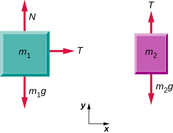
A block rests on the table, as shown. A light rope is attached to it and runs over a pulley. The other end of the rope is attached to a second block. The two blocks are said to be coupled. Block m₂ exerts a force due to its weight, which causes the system (two blocks and a string) to accelerate.

Strategy

We assume that the string has no mass so that we do not have to consider it as a separate object. Draw a free-body diagram for each block.

Solution

Significance

Each block accelerates (notice the labels shown for \(\vec{a}_{1}\) and \(\vec{a}_{2}\)); however, assuming the string remains taut, they accelerate at the same rate. Thus, we have |\(\vec{a}_{1}\)| = |\(\vec{a}_{2}\)|. If we were to continue solving the problem, we could simply call the acceleration \(\vec{a}\). Also, we use two free-body diagrams because we are usually finding tension T, which may require us to use a system of two equations in this type of problem. The tension is the same on both m₁ and m₂.

Exercise \(\PageIndex{1}\)

1. Draw the free-body diagram for the situation shown.
2. Redraw it showing components; use x-axes parallel to the two ramps.

Example \(\PageIndex{7}\)

Figure \(\PageIndex{8}\): Two connected blocks sliding down an inclined plane.

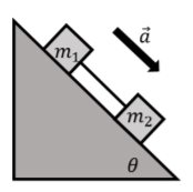
Two blocks, of masses \(m_{1}\) and \(m_{2}\), are placed on an inclined plane that makes an angle \(?\) with the horizontal. The blocks are connected by a massless string, as shown in Figure \(\PageIndex{8}\). The two blocks are sliding and accelerating downwards with an acceleration, \(\vec a\), as shown. The coefficient of kinetic friction between the plane and either block is \(µ_{k}\). Draw a free-body diagram for each block.

Solution

First, we identify the forces on each mass (each block), which we then use to make the free-body diagram shown in Figure \(\PageIndex{8}\). On mass \(m_1\), the forces are:

1. \(\vec F_{g1}\), its weight.
2. \(\vec N_1\), a normal force exerted by the inclined plane.
3. \(\vec f_{k1}\), a force of kinetic friction exerted by the inclined plane. The force is in the opposite direction of the motion, and has a magnitude given by \(f_{k1}=\mu_kN_1\).
4. \(\vec T\), a force of tension from the string.

On mass \(m_2\), the forces are:

1. \(\vec F_{g2}\), its weight.
2. \(\vec N_2\), a normal force from the inclined plane.
3. \(\vec f_{k2}\), a force of kinetic friction exerted by the inclined plane. The force is in the opposite direction of the motion, and has a magnitude given by \(f_{k2}=\mu_kN_2\).
4. \(-\vec T\), a force of tension from the string. This is the same force as on \(m_1\), but in the opposite direction. We chose to label the force as \(-\vec T\), instead of using a different variable, since it is just the negative of the vector that represents the tension force on \(m_1\).

In Figure \(\PageIndex{9}\), we have shown the forces on each block using a free-body diagram. We also reproduced the vector for the acceleration (we drew the vector for the acceleration using a thicker arrow to indicate that it has a different dimension). We also reproduced the angle \(\theta\) in the free-body diagram, as this is helpful once the free-body diagram is used with Newton’s Second Law.

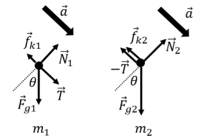
Figure \(\PageIndex{8}\).

 

The following example shows how to write Newton’s Second Law for a system of two blocks.

Example \(\PageIndex{8}\)

Figure \(\PageIndex{11}\): Two blocks connected by a massless string and massless pulley. Both blocks are accelerating.

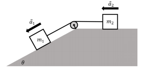
A block of mass \(m_1\) is placed on an incline that makes an angle of \(\theta\) with the horizontal. The block of mass \(m_1\) is connected by a massless string through a massless pulley to a second block of mass \(m_2\), which rests on a horizontal surface. The blocks are accelerating in such a way that the block of mass \(m_1\) is accelerating down the incline, as shown in Figure \(\PageIndex{5}\). The coefficient of kinetic friction between either block and the surface it is resting on is \(\mu_k\). Write Newton’s Second Law for both blocks.

Solution

First, we identify the forces on each mass (each block). On mass \(m_1\), the forces are:

1. \(\vec F_{g1}\), its weight.
2. \(\vec N_1\), a normal force exerted by the inclined plane.
3. \(\vec f_{k1}\), a force of kinetic friction exerted by the inclined plane. The force is in the opposite direction of the motion, and has a magnitude given by \(f_{k1}=\mu_kN_1\).
4. \(\vec T_1\), a force of tension from the string.

On mass \(m_2\), the forces are:

1. \(\vec F_{g2}\), its weight.
2. \(\vec N_2\), a normal force from the horizontal surface.
3. \(\vec f_{k2}\), a force of kinetic friction exerted by the horizontal surface. The force is in the opposite direction of the motion, and has a magnitude given by \(f_{k2}=\mu_kN_2\).
4. \(\vec T_2\), a force of tension from the string. This force has the same magnitude as the tension force \(\vec T_1\) exerted on mass \(m_1\), because the pulley is massless.

We can then proceed to draw the free-body diagram for each mass, and use that to write out Newton’s Second Law. For mass \(m_1\), the free-body diagram is shown in Figure \(\PageIndex{12}\). We have chosen a coordinate system that has the \(x\) axis parallel to the acceleration of the block, and the \(y\) axis upwards and perpendicular to the \(x\) axis, as shown.

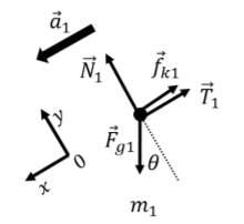
Figure \(\PageIndex{12}\): Free-body diagram for \(m_{1}\).

For \(m_1\), we can write Newton’s Second Law, starting with the \(x\) components: \[\begin{aligned} \sum F_x = F_{g1}\sin\theta-f_{k1}-T_1&=m_1a_1\\ \therefore m_1 g\sin\theta -\mu_k N_1 - T_1 &= m_1 a_1\end{aligned}\] where, in the second line, we used the magnitude of the weight (\(F_{g1}=m_1g\)) and of the force of kinetic friction (\(f_{k1}=\mu_kN_1\)). For the \(y\) component of Newton’s Second Law, in which the acceleration has no component, we have: \[\begin{aligned} \sum F_y = N_1 - F_{g1}\cos\theta &= 0\\ \therefore N_1=m_1g\cos\theta\end{aligned}\] which shows us that the magnitude of the normal force can easily be expressed in terms of the weight (\(F_{g1}=m_1g\)) and the angle of the incline.

For \(m_2\), we can proceed in much the same way, choosing a different coordinate system, since the acceleration vector for \(m_2\) points in a different direction (we don’t have to choose a different coordinate system, but we can if we find it makes things easier). The free-body diagram for \(m_2\) is shown in Figure \(\PageIndex{13}\) along with our choice of coordinate system.

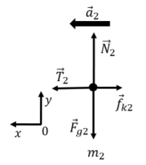
Figure \(\PageIndex{13}\): Free-body diagram for \(m_{2}\).

We start by writing out the \(x\) component of Newton’s Second Law for \(m_2\): \[\begin{aligned} \sum F_x = T_2 - f_{k2} &= m_2 a_2\\ \therefore T_2 - \mu_k N_2 = m_2 a_2\end{aligned}\] where again, we expressed the kinetic force of friction using the normal force and the coefficient of kinetic friction. The \(y\) component of Newton’s Second Law gives: \[\begin{aligned} \sum F_y = F_{g2}-N_2 &=0\\ \therefore N_2 = m_2g\end{aligned}\] where again, we expressed the weight in terms of the mass and \(g\), and we find that the normal force has the same magnitude as the weight.

Now that we have written Newton’s Second Law for each mass, we can write all four equations that we obtained to describe the system of two masses. We should also note that the magnitude of the tension forces are the same for the two masses (\(T_1=T_2=T\)), and that since the masses are connected by a string, the magnitude of their acceleration vectors are the same (\(a_1=a_2=a\)). Using this, we can describe the full system with the following 4 equations: \[\begin{aligned} m_1 g\sin\theta -\mu_k N_1 - T &= m_1 a\\ N_1=m_1g\cos\theta\\ T - \mu_k N_2 = m_2 a\\ N_2 = m_2g\end{aligned}\] Of the variables above (\(m_1\), \(m_2\), \(\mu_k\), \(T\), \(N_1\), \(N_2\), \(a\)), one would only need to specify all but four of them to fully describe the motion of the system. For example, if one specifies the two masses and the coefficient of kinetic friction, all of the other variables can be determined.