6.7: Motion in a Curved Path

Learning Objectives

• Explain the equation for centripetal acceleration
• Apply Newton’s second law to develop the equation for centripetal force
• Use circular motion concepts in solving problems involving Newton’s laws of motion

Flat Curves

We have previously examined the basic concepts of circular motion. An object undergoing circular motion, must be accelerating because it is changing the direction of its velocity. We proved that this centrally directed acceleration, called centripetal acceleration, is given by the formula

\[\vec a_{c} = - \frac{v^{2}}{r} \hat{r}\]

where \(v\) is the velocity of the object, directed along a tangent line to the curve at any instant. If we know the angular velocity \(\omega\), then we can use

\[\vec a_{c} = - r \omega^{2} \hat{r} \ldotp\]

Angular velocity gives the rate at which the object is turning through the curve, in units of rad/s. This acceleration acts along the radius of the curved path and is thus also referred to as a radial acceleration.

An acceleration must be produced by a force. Any force or combination of forces can cause a centripetal or radial acceleration. Just a few examples are the tension in the rope on a tether ball, the force of Earth’s gravity on the Moon, friction between roller skates and a rink floor, a banked roadway’s force on a car, and forces on the tube of a spinning centrifuge. Any net force causing uniform circular motion is called a centripetal force. The direction of a centripetal force is toward the center of curvature, the same as the direction of centripetal acceleration. According to Newton’s second law of motion, net force is mass times acceleration: \(\vec F_{net} = m\vec a\). For uniform circular motion, the acceleration is the centripetal acceleration: \(\vec a = \vec a_c\). Thus, the magnitude of centripetal force \(\vec F_c\) is

\[\vec F_{c} = m\vec a_{c} \ldotp\]

By substituting the expressions for centripetal acceleration a_c (\(\vec a_{c} =- \frac{v^{2}}{r} \hat{r}; \vec a_{c} = - r \omega^{2} \hat{r}\)), we get two expressions for the centripetal force \(\vec F_{c}\) in terms of mass, velocity, angular velocity, and radius of curvature:

\[\vec F_{c} = - m \frac{v^{2}}{r} \hat{r}; \quad F_{c} =- m r\omega^{2} \hat{r} \ldotp \label{6.3}\]

You may use whichever expression for centripetal force is more convenient. Centripetal force \(\vec{F}_{c}\) is always perpendicular to the path and points to the center of curvature, because \(\vec{a}_{c}\) is perpendicular to the velocity and points to the center of curvature. 

Example \(\PageIndex{1}\): What Coefficient of Friction Do Cars Need on a Flat Curve?

1. Calculate the centripetal force exerted on a 900.0-kg car that negotiates a 500.0-m radius curve at 25.00 m/s.
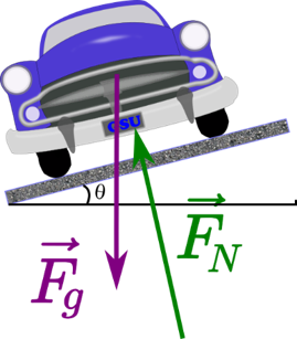
2. Assuming an unbanked curve, find the minimum static coefficient of friction between the tires and the road, static friction being the reason that keeps the car from slipping (Figure \(\PageIndex{2}\)).

Solution

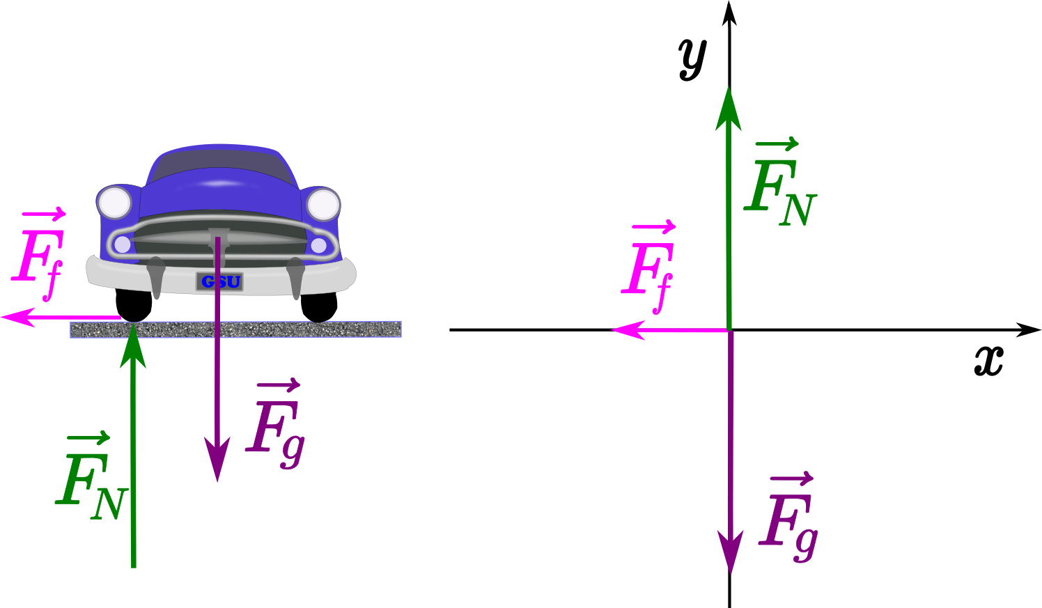
Figure \(\PageIndex{2}\): This car on level ground is moving away and turning to the left. The centripetal force causing the car to turn in a circular path is due to friction between the tires and the road. A minimum coefficient of friction is needed, or the car will move in a larger-radius curve and leave the roadway.

a) We know that \(F_{c} = m \frac{v^{2}}{r}\). Thus \(F_{c} = m \frac{v^{2}}{r} = \frac{(900.0\; kg)(25.00\; m/s)^{2}}{(500.0\; m)} = 1125\; N \)

b) Figure \(\PageIndex{2}\) shows the forces acting on the car on an unbanked (level ground) curve. Writing Newton's Second Law of motion:
\[\vec{F}_f + \vec{F}_N + \vec{F}_g = m \vec{a} \]

Resolving the equation along the \(x\) and \(y\) directions:

along \(x\): \[-F_f + 0 + 0 = - m a_c \]

along \(y\): \[0 + F_N - F_g = 0 \]

Friction is to the left, keeping the car from slipping, and because it is the only horizontal force acting on the car, the friction is the centripetal force in this case. We know that the maximum static friction (at which the tires roll but do not slip) is \(\mu_{s} F_N\), where \(\mu_{s}\) is the static coefficient of friction and \(F_N\) is the normal force. As can be seen from the \(y\)-axis expression of Newton's second law of motion, the normal force equals the car’s weight: \( F_N = F_g = m g\)

On the other hand, from  the \(x\)-axis expression of Newton's second law of motion, we get:  \(F_{f} = m a_c = m \frac{v^{2}}{r}\)

We also know that: \(F_{f} = \mu_{s} F_{N}\)

Combining these 3 equations: \(F_{f} = \mu_{s} F_{N}= \mu_{s} mg \) and \(F_{f} = m \frac{v^{2}}{r}\)

Thus: \(m \frac{v^{2}}{r} = \mu_{s} mg \)

and, noting that mass cancels, \(\frac{v^{2}}{r} = \mu_{s} g\)

Substituting the knowns, \(\mu_{s} = \frac{(25.00\; m/s)^{2}}{(500.0\; m)(9.80\; m/s^{2})} = 0.13 \)(Because coefficients of friction are approximate, the answer is given to only two digits.)

Discussion

The coefficient of friction found in Figure \(\PageIndex{2b}\) is much smaller than is typically found between tires and roads. The car still negotiates the curve if the coefficient is greater than 0.13, because static friction is a responsive force, able to assume a value less than but no more than \(\mu_{s}\)N. A higher coefficient would also allow the car to negotiate the curve at a higher speed, but if the coefficient of friction is less, the safe speed would be less than 25 m/s. Note that mass cancels, implying that, in this example, it does not matter how heavily loaded the car is to negotiate the turn. Mass cancels because friction is assumed proportional to the normal force, which in turn is proportional to mass. If the surface of the road were banked, the normal force would be less, as discussed next.

 

Example \(\PageIndex{2}\)

Figure \(\PageIndex{6}\): A ball attached to a string undergoing circular motion in a vertical plane.

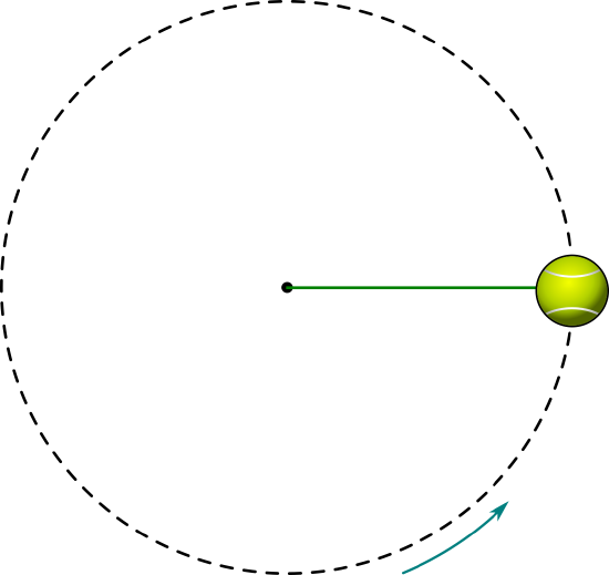
A ball is attached to a mass-less string and executing circular motion along a circle of radius \(R\) that is in the vertical plane, as depicted in Figure \(\PageIndex{6}\). Can the speed of the ball be constant? What is the minimum speed of the ball at the top of the circle if it is able to make it around the circle?

Solution

The forces that are acting on the ball are:

1. \(\vec F_g\), its weight with magnitude \(mg\).
2. \(\vec F_T\), a force of tension exerted by the string.

Figure \(\PageIndex{7}\) shows the free-body diagram for the forces on the ball at three different locations along the path of the circle.

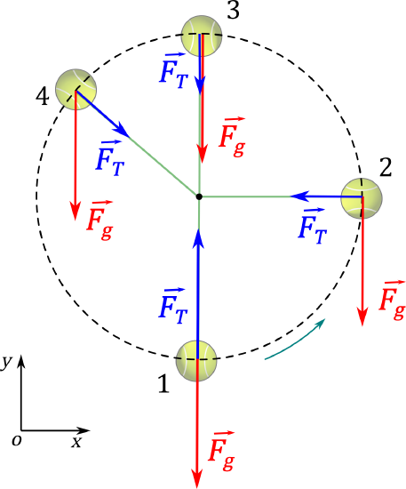
Figure \(\PageIndex{7}\): A ball attached to a string undergoing circular motion in a vertical plane.

In order for the ball to go around in a circle, there must be at least a component of the net force on the ball that is directed towards the center of the circle at all times.

Consider in particular the position when the string is horizontal. The free-body diagram in Figure \(\PageIndex{7}\) shows  the weight and tension. The vector sum, the net force, which points downwards and to the left. It is thus clearly impossible for the acceleration vector to point towards the center of the circle, and the acceleration will have components that are both tangential (\(\vec a_T\)) to the circle and radial (\(\vec a_R\)). Note that the direction of (\(\vec a_T\)) for that position is (\(\hat a_T = -\hat \theta = - \hat j\)) and that the direction of (\(\vec a_R\)) for that position is (\(\hat a_R = -\hat r = - \hat i\)).

The radial component of the acceleration will change the direction of the velocity vector so that the ball remains on the circle, and the tangential component will reduce the magnitude of the velocity vector. According to our model, it is thus impossible for the ball to go around the circle at constant speed, and the speed must decrease as it goes from the bottom to the top, no matter how one pulls on the string (you can convince yourself of this by drawing the free-body diagram at any point in between).

The minimum speed for the ball at the top of the circle is given by the condition that the tension in the string is zero just at the top of the trajectory. The ball can still go around the circle because, at that position, gravity is towards the center of the circle and can thus give an acceleration that is radial, even with no tension. The \(y\) component of Newton’s Second Law, at that position gives:

\[\begin{aligned} \sum F_y = -F_g &= ma_y\\ \therefore a_y &=-g\end{aligned}\]

The magnitude of the acceleration is the radial acceleration, and is thus related to the speed at the top of the trajectory:

\[\begin{aligned} a_R&=-a_y=g = m\frac{v^2}{R}\\ \therefore v_{min}&=\sqrt{\frac{gR}{m}}\end{aligned}\]

which is the minimum speed at the top of the trajectory for the ball to be able to continue along the circle. The tension in the string would change as the ball moves around the circle, and will be highest at the bottom of the trajectory, since the tension has to be bigger than gravity so that the net force at the bottom of the trajectory is upwards (towards the center of the circle).

Discussion:

The model for the minimum speed of the ball at the top of the circle makes sense because:

• \(\sqrt{\frac{gR}{m}}\) has the dimension of speed.
• The minimum velocity is larger if the circle has a larger radius (try this with a mass attached at the end of a string).
• The minimum velocity is larger if the mass is bigger (again, try this at home!).

Example \(\PageIndex{3}\)

Figure \(\PageIndex{3}\): A toy rocket accelerating around a circle of radius \(R\), as seen from above.

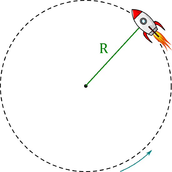
A toy rocket is attached to a string on a horizontal frictionless table, as shown in Figure \(\PageIndex{3}\). The rocket has a mass \(m\) and produces a constant force of thrust with a magnitude \(\vec{F}\) that accelerates the rocket along a circle of radius \(R\) (the length of the string). If the rocket starts at rest, what distance along the circumference of the circle will the rocket have traveled after a time, \(t\)?

Solution

We can model the rocket as a point particle of mass \(m\) with the following forces exerted on it:

1. \(\vec F\), the thrust of the rocket, always acting tangent to the circle.
2. \(\vec F_T\), the force of tension in the string, always acting towards the center of the circle.
3. \(\vec F_g\), the rocket’s weight, acting perpendicular to the table in the downward direction (into the page), with magnitude \(mg\).
4. \(\vec F_N\), a normal force exerted by the table, acting perpendicular to the table in the downward direction (out of the page), with magnitude \(mg\).

Writing Newton's second law of motion,

\[\vec F_{net} = \vec F_T + \vec F + \vec F_g + \vec F_N\]

Because the normal force and the weight are equal in magnitude and opposite in direction (\(|\vec F_g| = |\vec F_N|\)), the net force will be the sum of the force of thrust and the force of tension, which are always perpendicular to each other.

\[\vec F_{net} = \vec F_T + \vec F = m\vec a\label{N2L}\]

Thinking about this with Newton’s Second Law, we could model the force of thrust as increasing the speed of the particle, while the force of tension keeps the rocket moving in a circle (it cannot increase the speed, since it is always perpendicular to the motion).

We use the polar coordinate system whose origin coincides with the center of the rocket, as shown in Figure \(\PageIndex{4}\). The force of thrust and the tension are also shown in the diagram. Assume that the position shown for the the rocket corresponds to time, \(t=0\).

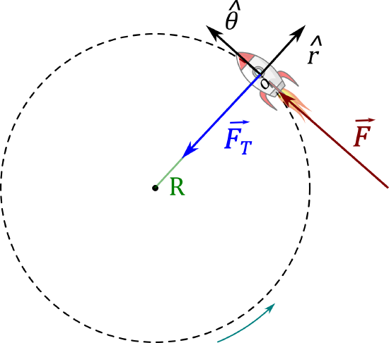
Figure \(\PageIndex{4}\): Coordinate system to describe the motion of the rocket.

 

We can rewrite Equation \ref{N2L} as:

\[\begin{aligned} \vec F_T + \vec F = m (\vec a_c + \vec a_T)\end{aligned}\]

where \(\vec a_T\) is the acceleration along the tangential direction \(\hat\theta\), and \(\vec a_c\) is the acceleration along the radial direction \(\hat r\). Resolving our equation along both directions:

along \(\hat\theta\): \(\begin{aligned} 0 + F = m (0 +  a_T)\end{aligned}\)

and along \(\hat r\): \(\begin{aligned} - F_T + 0 = m (- a_c +  0)\end{aligned}\)

note that both \(\vec F_T\) and \(\vec a_c\) point in the negative direction of \(\hat r\).

The equation along \(\hat\theta\) provides the tangential acceleration:

\[\begin{aligned}  a_T = \frac{F} {m}\end{aligned}\]

Which allows us to determine the angular acceleration:

\[\begin{aligned} \alpha &= \frac{a_T}{R} = \frac{F}{mR}\end{aligned}\]

This indicates that the rocket is accelerating in the counter-clockwise direction about the normal to the circle.

After a period of time \(t\), the rocket will have covered an angular displacement, \(\Delta \theta\), given by:

\[\begin{aligned} \Delta \theta &= \theta(t)-\theta_0 = \omega_0t + \frac{1}{2}\alpha t^2\\ &=\frac{1}{2}\frac{F}{mR} t^2\end{aligned}\]

The linear displacement, \(\Delta s\), that corresponds to this angular displacement is:

\[\begin{aligned} \Delta s = R \Delta\theta = \frac{1}{2}\frac{F}{m} t^2\end{aligned}\]

Discussion

The formula that we found for the total linear displacement is the same that we would have found if the particle were moving in a straight line with a net force \(F\) applied to it (as the particle would have a constant acceleration given by \(F/m\)).

Banked Curves

Let us now consider banked curves, where the slope of the road helps you negotiate the curve (Figure \(\PageIndex{3}\)). The greater the angle ? , the faster you can take the curve. Race tracks for bikes as well as cars, for example, often have steeply banked curves. In an “ideally banked curve,” the angle \(\theta\) is such that you can negotiate the curve at a certain speed without the aid of friction between the tires and the road. We will derive an expression for \(\theta\) for an ideally banked curve and consider an example related to it.

Figure \(\PageIndex{3}\): The car on this banked curve is moving towards and turning to the right of the driver.

Figure \(\PageIndex{5}\): The Free body digram for the car. Note that the x-axis is chosen parallel to the centripetal acceleration.

For ideal banking, the net external force equals the horizontal centripetal force in the absence of friction. The components of the normal force \(\vec{F}_N\) in the horizontal and vertical directions must equal the centripetal force and the weight of the car, respectively. In cases in which forces are not parallel, it is most convenient to consider components along perpendicular axes—in this case, the vertical and horizontal directions. One of the axis, should be chosen parallel to the acceleration.

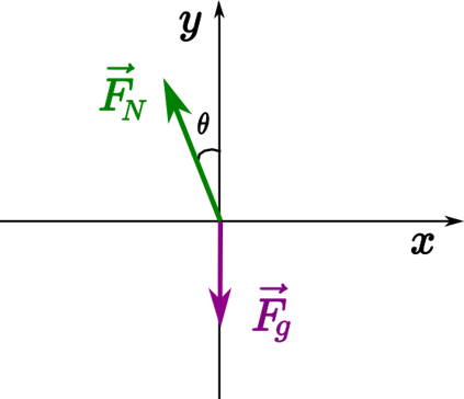
Figure \(\PageIndex{5}\) shows a free-body diagram for a car on a frictionless banked curve. If the angle \(\theta\) is ideal for the speed and radius, then the net external force \(\vec{F}_{net}\) equals the necessary centripetal force. The only two external forces acting on the car are its weight \(\vec{F}_g\) and the normal force of the road \(\vec{F}_N\). (A frictionless surface can only exert a force perpendicular to the surface—that is, a normal force.)

\[\vec{F}_N + \vec{F}_g = \vec{F}_{net} = m \vec{a}_c \ldotp\]

Resolving the equation along the x-axis,

\[- F_N \sin \theta = - \frac{mv^{2}}{r} \ldotp\]

Resolving the equation along the y-axis,

\[F_N \cos \theta - F_g = 0 \Longrightarrow F_N \cos \theta = F_g = m g \ldotp\]

Now we can combine these two equations to eliminate \(F_N\) and get an expression for \(\theta\). Solving the second equation for \(F_N = \frac{mg}{\cos \theta}\) and substituting this into the first yields

\[\begin{split} \frac{mg}{\cos \theta} \sin \theta = mg \frac{\sin \theta}{\cos \theta} & = \frac{mv^{2}}{r} \\ mg \tan \theta & = \frac{mv^{2}}{r} \\ \tan \theta & = \frac{v^{2}}{rg} \ldotp \end{split}\]

Taking the inverse tangent gives

\[\theta = \tan^{-1} \left(\dfrac{v^{2}}{rg}\right) \ldotp \label{6.4}\]

This expression can be understood by considering how \(\theta\) depends on \(v\) and \(r\). A large \(\theta\) is obtained for a large \(v\) and a small \(r\). That is, roads must be steeply banked for high speeds and sharp curves. Friction helps, because it allows you to take the curve at greater or lower speed than if the curve were frictionless. Note that \(\theta\) does not depend on the mass of the vehicle.

Example \(\PageIndex{4}\): What Is the Ideal Speed to Take a Steeply Banked Tight Curve?

Curves on some test tracks and race courses, such as Daytona International Speedway in Florida, are very steeply banked. This banking, with the aid of tire friction and very stable car configurations, allows the curves to be taken at very high speed. To illustrate, calculate the speed at which a 100.0-m radius curve banked at 31.0° should be driven if the road were frictionless.

Strategy

We first note that all terms in the expression for the ideal angle of a banked curve except for speed are known; thus, we need only rearrange it so that speed appears on the left-hand side and then substitute known quantities.

Solution

Starting with

\[\tan \theta = \frac{v^{2}}{rg},\]

we get

\[v = \sqrt{rg \tan \theta} \ldotp\]

Noting that tan 31.0° = 0.609, we obtain

\[v = \sqrt{(100.0\; m)(9.80\; m/s^{2})(0.609)} = 24.4\; m/s \ldotp\]

Significance

This is just about 165 km/h, consistent with a very steeply banked and rather sharp curve. Tire friction enables a vehicle to take the curve at significantly higher speeds.

Airplanes also make turns by banking. The lift force, due to the force of the air on the wing, acts at right angles to the wing. When the airplane banks, the pilot is obtaining greater lift than necessary for level flight. The vertical component of lift balances the airplane’s weight, and the horizontal component accelerates the plane. The banking angle shown in Figure \(\PageIndex{4}\) is given by \(\theta\). We analyze the forces in the same way we treat the case of the car rounding a banked curve.

Figure \(\PageIndex{4}\): In a banked turn, the horizontal component of lift is unbalanced and accelerates the plane. The normal component of lift balances the plane’s weight. The banking angle is given by \(\theta\). Compare the vector diagram with that shown in Figure 6.22.

Note

A circular motion requires a force, the so-called centripetal force, which is directed to the axis of rotation.

Non-uniform circular motion

In non-uniform circular motion, an object’s motion is along a circle, but the object’s speed is not constant. In particular, the following will be true

• The object’s velocity vector is always tangent to the circle. It can be written as \(\vec v_T\).
• The speed and angular speed of the object are not constant.
• The angular acceleration \(\vec \alpha\) of the object is not zero.
• The acceleration vector will not point towards the center of the circle.

Since the acceleration vector does not point towards the center of the circle, it is usually convenient to break up the acceleration vector into two components: \(\vec a_R\), a component that is radial (towards the center of the circle), and \(\vec a_T\), a component that is tangent to the circle (and perpendicular to to the radial component). The radial component is “responsible” for the change in direction of the velocity such that the object goes in a circle. the magnitude of the radial acceleration is the same as it is for uniform circular motion:

\[\begin{aligned} \vec a_R= - \frac{v_T^2(t)}{r} \hat{r}\end{aligned}\]

where the speed is no longer constant in time. The tangential component of the acceleration is responsible for changing the magnitude of the velocity of the object:

\[\begin{aligned} \vec a_T = \frac{d\vec v_T(t)}{dt}\end{aligned}\]

The overall acceleration is then,

\[\begin{aligned}\vec a = \vec a_R+\vec a_T = - \frac{v_T^2(t)}{r} \hat{r}+\frac{d\vec v_T(t)}{dt}\end{aligned}\]

Example \(\PageIndex{5}\)

Figure \(\PageIndex{1}\): An ant on a horizontal turntable that is starting to spin, as seen from above.

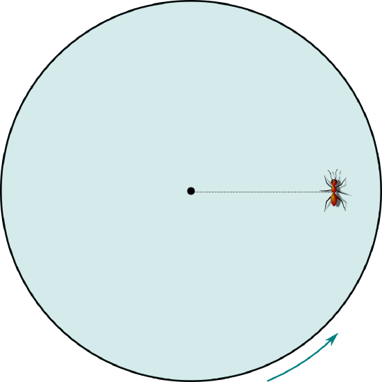
A small ant is sleeping on a turntable just as the turntable starts to spin from rest, with an angular acceleration \(\alpha=1\text{rad/s}^{2}\) that is small enough so that, initially, the ant remains on the turntable. The ant is a distance \(R=0.1\text{m}\) from the center of the turntable, as shown in Figure \(\PageIndex{1}\) and the coefficient of static friction between the ant’s “feet” and the turntable is \(\mu_s=0.5\). After how much time will the ant slide off from the turntable?

Solution

As the turntable accelerates, the force of static friction between the turntable and the ant will keep the ant moving with the turntable. Once the turntable is going fast enough, the force of friction will no longer be large enough to provide the total acceleration that is required to keep the ant moving with the turntable (with a constant tangential component of the acceleration and an increasing radial component of the acceleration).

The forces on the ant are:

1. \(\vec F_g\), its weight, with magnitude \(mg\).
2. \(\vec F_N\), a normal force exerted by the turntable on the ant.
3. \(\vec F_{fs}\), a force of static friction exerted by the turntable on the ant. The force of friction will be such that it has both radial and tangential components.

A free-body diagram for the forces on the ant is shown in Figure 6.4.2, as seen from above and from the side, for some point in time. We have chosen the point in time to be just when the ant is about to slide off of the turntable, when the force of static friction makes an unknown angle \(\theta\) with the \(x\) axis. We have placed the origin of the coordinate system at the center of the turntable and chosen the \(x\) axis such that the ant is located on the positive \(x\) axis with its velocity in the positive \(y\) direction. We used a three dimensional coordinate system where the weight and normal force are exerted in the \(z\) (vertical) direction since the acceleration vector of the ant will have both radial (\(x\)) and tangential (\(y\)) components.

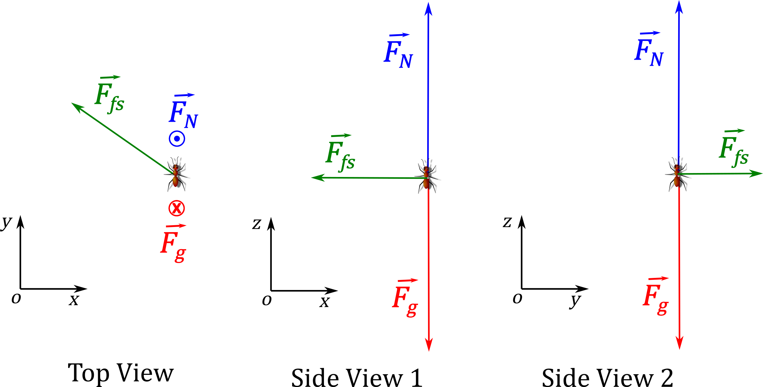
Figure \(\PageIndex{2}\): (Left:) Forces on the ant as seen from above. The normal force \(\vec F_N\) is out of the page \((\odot )\), whereas the weight \(\vec F_g\) is into the page \((×)\). (Center and Right:) Forces on the ant as seen from the side. Note that the force of static friction \(\vec F_{f_s}\)has components in the \(x\) and \(y\) directions, which is why their magnitude is shown as being smaller than in the top view.

Writing Newton’s Second Law for the three forces acting on the ant:

\[\begin{aligned}\sum \vec F_{ext} &=\vec F_{net} &= \vec F_{N} + \vec F_g + \vec F_{fs}\end{aligned}\]

The \(z\) component relates the weight and normal force:

\[\begin{aligned}\sum F_z &= F_{N} - F_g = 0\\ \therefore F_{N}&=mg\end{aligned}\]

The \(x\) component of Newton’s Second Law is such that the \(x\) component of the acceleration is its radial component:

\[\begin{aligned} \sum F_x &= -F_{fs}\cos\theta = -ma_R = -m\frac{v^2}{R} \\ \therefore F_{fs}\cos\theta &= m\frac{v^2}{R} \end{aligned}\]

The \(y\) component of Newton’s Second relates the tangential component of the force of static friction to the tangential component of the acceleration:

\[\begin{aligned} \sum F_y &=F_{fs}\sin\theta = ma_T \\ \therefore F_{fs}\sin\theta &= m\alpha R\end{aligned}\]

where we used the fact that the (linear) tangential acceleration, \(a_T\), is related to the angular acceleration, \(\alpha\), by:

\[\begin{aligned} a_T = \alpha R\end{aligned}\]

Summarizing the three equations that we obtained from the three components of Newton’s Second Law:

\[\begin{aligned} F_{fs}\cos\theta &= m\frac{v^2}{R}\\ F_{fs}\sin\theta &= m\alpha R\\ F_{N}&=mg\end{aligned}\]

Also, note that the speed, \(v(t)\) at some time \(t\) is given by simple kinematics:

\[\begin{aligned} v(t)=v_0+a_Tt=(0)+\alpha R t\end{aligned}\]

The ant will start to slip when the force of friction reaches its maximal amplitude, \(F_{fs}=\mu_s F_N=\mu_S mg\). The \(x\) of Newton’s Second Law can be used to find an expression for the time at which force of friction reaches its maximal value (in terms of the unknown angle \(\theta\)):

\[\begin{aligned} F_{fs}\cos\theta &= m\frac{v^2}{R}\\ \mu_sg\cos\theta &= R\alpha^2t^2\\ \therefore t &= \sqrt{\frac{\mu_sg\cos\theta}{R\alpha^2}}\end{aligned}\]

We can use the \(y\) component to determine the angle \(\theta\):

\[\begin{aligned} F_{fs}\sin\theta &= m\alpha R\\ \mu_sg\sin\theta &= \alpha R\\ \therefore \sin\theta &= \frac{\alpha R}{\mu_s g}\\ \therefore \theta &= \sin^{-1}\left( \frac{\alpha R}{\mu_s g} \right)=\sin^{-1}\left( \frac{(1\text{rad/s}^{2})(0.1\text{m})}{(0.5)(9.8\text{N/kg})} \right)\\ &=1.17^{\cdot}\end{aligned}\]

The angle is very small, and we see that the force of friction is mostly directed towards the center of the circle. The radial acceleration is thus much larger than the tangential acceleration. We can then use the angle to find the time using the expression we derived above:

\[\begin{aligned} t &= \sqrt{\frac{\mu_sg\cos\theta}{R\alpha^2}}= \sqrt{\frac{(0.5)(9.8\text{N/kg})\cos(1.17^{\cdot})}{(0.1\text{m})(1\text{rad/s}^{2})^2}}\\ &=7.0\text{s}\end{aligned}\]

Inertial Forces and Noninertial (Accelerated) Frames: The Coriolis Force

What do taking off in a jet airplane, turning a corner in a car, riding a merry-go-round, and the circular motion of a tropical cyclone have in common? Each exhibits inertial forces—forces that merely seem to arise from motion, because the observer’s frame of reference is accelerating or rotating. When taking off in a jet, most people would agree it feels as if you are being pushed back into the seat as the airplane accelerates down the runway. Yet a physicist would say that you tend to remain stationary while the seat pushes forward on you. An even more common experience occurs when you make a tight curve in your car—say, to the right (Figure \(\PageIndex{5}\)). You feel as if you are thrown (that is, forced) toward the left relative to the car. Again, a physicist would say that you are going in a straight line (recall Newton’s first law) but the car moves to the right, not that you are experiencing a force from the left.

Figure \(\PageIndex{5}\): (a) The car driver feels herself forced to the left relative to the car when she makes a right turn. This is an inertial force arising from the use of the car as a frame of reference. (b) In Earth’s frame of reference, the driver moves in a straight line, obeying Newton’s first law, and the car moves to the right. There is no force to the left on the driver relative to Earth. Instead, there is a force to the right on the car to make it turn.

We can reconcile these points of view by examining the frames of reference used. Let us concentrate on people in a car. Passengers instinctively use the car as a frame of reference, whereas a physicist might use Earth. The physicist might make this choice because Earth is nearly an inertial frame of reference, in which all forces have an identifiable physical origin. In such a frame of reference, Newton’s laws of motion take the form given in Newton’s Laws of Motion. The car is a noninertial frame of reference because it is accelerated to the side. The force to the left sensed by car passengers is an inertial force having no physical origin (it is due purely to the inertia of the passenger, not to some physical cause such as tension, friction, or gravitation). The car, as well as the driver, is actually accelerating to the right. This inertial force is said to be an inertial force because it does not have a physical origin, such as gravity.

A physicist will choose whatever reference frame is most convenient for the situation being analyzed. There is no problem to a physicist in including inertial forces and Newton’s second law, as usual, if that is more convenient, for example, on a merry-go-round or on a rotating planet. Noninertial (accelerated) frames of reference are used when it is useful to do so. Different frames of reference must be considered in discussing the motion of an astronaut in a spacecraft traveling at speeds near the speed of light, as you will appreciate in the study of the special theory of relativity.

Let us now take a mental ride on a merry-go-round—specifically, a rapidly rotating playground merry-go-round (Figure \(\PageIndex{6}\)). You take the merry-go-round to be your frame of reference because you rotate together. When rotating in that noninertial frame of reference, you feel an inertial force that tends to throw you off; this is often referred to as a centrifugal force (not to be confused with centripetal force). Centrifugal force is a commonly used term, but it does not actually exist. You must hang on tightly to counteract your inertia (which people often refer to as centrifugal force). In Earth’s frame of reference, there is no force trying to throw you off; we emphasize that centrifugal force is a fiction. You must hang on to make yourself go in a circle because otherwise you would go in a straight line, right off the merry-go-round, in keeping with Newton’s first law. But the force you exert acts toward the center of the circle.

Figure \(\PageIndex{6}\): (a) A rider on a merry-go-round feels as if he is being thrown off. This inertial force is sometimes mistakenly called the centrifugal force in an effort to explain the rider’s motion in the rotating frame of reference. (b) In an inertial frame of reference and according to Newton’s laws, it is his inertia that carries him off (the unshaded rider has F_net = 0 and heads in a straight line). A force, F_centripetal, is needed to cause a circular path.

This inertial effect, carrying you away from the center of rotation if there is no centripetal force to cause circular motion, is put to good use in centrifuges (Figure \(\PageIndex{7}\)). A centrifuge spins a sample very rapidly, as mentioned earlier in this chapter. Viewed from the rotating frame of reference, the inertial force throws particles outward, hastening their sedimentation. The greater the angular velocity, the greater the centrifugal force. But what really happens is that the inertia of the particles carries them along a line tangent to the circle while the test tube is forced in a circular path by a centripetal force.

Figure \(\PageIndex{7}\): Centrifuges use inertia to perform their task. Particles in the fluid sediment settle out because their inertia carries them away from the center of rotation. The large angular velocity of the centrifuge quickens the sedimentation. Ultimately, the particles come into contact with the test tube walls, which then supply the centripetal force needed to make them move in a circle of constant radius.

Let us now consider what happens if something moves in a rotating frame of reference. For example, what if you slide a ball directly away from the center of the merry-go-round, as shown in Figure \(\PageIndex{8}\)? The ball follows a straight path relative to Earth (assuming negligible friction) and a path curved to the right on the merry-go-round’s surface. A person standing next to the merry-go-round sees the ball moving straight and the merry-go-round rotating underneath it. In the merry-go-round’s frame of reference, we explain the apparent curve to the right by using an inertial force, called the Coriolis force, which causes the ball to curve to the right. The Coriolis force can be used by anyone in that frame of reference to explain why objects follow curved paths and allows us to apply Newton’s laws in noninertial frames of reference.

Figure \(\PageIndex{8}\): Looking down on the counterclockwise rotation of a merry-go-round, we see that a ball slid straight toward the edge follows a path curved to the right. The person slides the ball toward point B, starting at point A. Both points rotate to the shaded positions (A’ and B’) shown in the time that the ball follows the curved path in the rotating frame and a straight path in Earth’s frame.

Up until now, we have considered Earth to be an inertial frame of reference with little or no worry about effects due to its rotation. Yet such effects do exist—in the rotation of weather systems, for example. Most consequences of Earth’s rotation can be qualitatively understood by analogy with the merry-go-round. Viewed from above the North Pole, Earth rotates counterclockwise, as does the merry-go-round in Figure \(\PageIndex{8}\). As on the merry-go-round, any motion in Earth’s Northern Hemisphere experiences a Coriolis force to the right. Just the opposite occurs in the Southern Hemisphere; there, the force is to the left. Because Earth’s angular velocity is small, the Coriolis force is usually negligible, but for large-scale motions, such as wind patterns, it has substantial effects.

The Coriolis force causes hurricanes in the Northern Hemisphere to rotate in the counterclockwise direction, whereas tropical cyclones in the Southern Hemisphere rotate in the clockwise direction. (The terms hurricane, typhoon, and tropical storm are regionally specific names for cyclones, which are storm systems characterized by low pressure centers, strong winds, and heavy rains.) Figure \(\PageIndex{9}\) helps show how these rotations take place. Air flows toward any region of low pressure, and tropical cyclones contain particularly low pressures. Thus winds flow toward the center of a tropical cyclone or a low-pressure weather system at the surface. In the Northern Hemisphere, these inward winds are deflected to the right, as shown in the figure, producing a counterclockwise circulation at the surface for low-pressure zones of any type. Low pressure at the surface is associated with rising air, which also produces cooling and cloud formation, making low-pressure patterns quite visible from space. Conversely, wind circulation around high-pressure zones is clockwise in the Southern Hemisphere but is less visible because high pressure is associated with sinking air, producing clear skies.

Figure \(\PageIndex{9}\): (a) The counterclockwise rotation of this Northern Hemisphere hurricane is a major consequence of the Coriolis force. (b) Without the Coriolis force, air would flow straight into a low-pressure zone, such as that found in tropical cyclones. (c) The Coriolis force deflects the winds to the right, producing a counterclockwise rotation. (d) Wind flowing away from a high-pressure zone is also deflected to the right, producing a clockwise rotation. (e) The opposite direction of rotation is produced by the Coriolis force in the Southern Hemisphere, leading to tropical cyclones. (credit a and credit e: modifications of work by NASA)

The rotation of tropical cyclones and the path of a ball on a merry-go-round can just as well be explained by inertia and the rotation of the system underneath. When noninertial frames are used, inertial forces, such as the Coriolis force, must be invented to explain the curved path. There is no identifiable physical source for these inertial forces. In an inertial frame, inertia explains the path, and no force is found to be without an identifiable source. Either view allows us to describe nature, but a view in an inertial frame is the simplest in the sense that all forces have origins and explanations.

Apparent Weight: Accounting for Earth’s Rotation

As we saw in Applications of Newton’s Laws, objects moving at constant speed in a circle have a centripetal acceleration directed toward the center of the circle, which means that there must be a net force directed toward the center of that circle. Since all objects on the surface of Earth move through a circle every 24 hours, there must be a net centripetal force on each object directed toward the center of that circle.

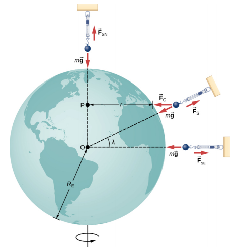
Let’s first consider an object of mass m located at the equator, suspended from a scale (Figure \(\PageIndex{3}\)). The scale exerts an upward force \(\vec{F}_{s}\) away from Earth’s center. This is the reading on the scale, and hence it is the apparent weight of the object. The weight (mg) points toward Earth’s center. If Earth were not rotating, the acceleration would be zero and, consequently, the net force would be zero, resulting in F_s = mg . This would be the true reading of the weight.

Figure \(\PageIndex{3}\): For a person standing at the equator, the centripetal acceleration (ac) is in the same direction as the force of gravity. At latitude \(\lambda\), the angle the between ac and the force of gravity is \(\lambda\) and the magnitude of ac decreases with \(\cos \lambda\).

With rotation, the sum of these forces must provide the centripetal acceleration, \(a_c\). Using Newton’s second law, we have

\[\sum F = F_{s} - mg = ma_{c} \quad where\; a_{c} = - \frac{v^{2}}{r} \ldotp \label{13.3}\]

Note that a_c points in the same direction as the weight; hence, it is negative. The tangential speed v is the speed at the equator and r is R_E. We can calculate the speed simply by noting that objects on the equator travel the circumference of Earth in 24 hours. Instead, let’s use the alternative expression for a_c from Motion in Two and Three Dimensions. Recall that the tangential speed is related to the angular speed (\(\omega\)) by v = r\(\omega\). Hence, we have a_c = -r\(\omega\)². By rearranging Equation 13.3 and substituting r = R_E, the apparent weight at the equator is

\[F_{s} = m (g - R_{E} \omega^{2}) \ldotp\]

The angular speed of Earth everywhere is

\[\omega = \frac{2 \pi\; rad}{24\; hr \times 3600\; s/hr} = 7.27 \times 10^{-5}\; rad/s \ldotp\]

Substituting for the values of R_E and \(\omega\), we have R_E\(\omega\)² = 0.0337 m/s². This is only 0.34% of the value of gravity, so it is clearly a small correction.

Example \(\PageIndex{6}\): Zero Apparent Weight

How fast would Earth need to spin for those at the equator to have zero apparent weight? How long would the length of the day be?

Strategy

Using Equation \ref{13.3}, we can set the apparent weight (F_s) to zero and determine the centripetal acceleration required. From that, we can find the speed at the equator. The length of day is the time required for one complete rotation.

Solution

From Equation \ref{13.2}, we have \(\sum\)F = F_s - mg = ma_c, so setting F_s = 0, we get g = a_c. Using the expression for a_c, substituting for Earth’s radius and the standard value of gravity, we get

\[\begin{split} a_{c} & = \frac{v^{2}}{r} = g \\ v & = \sqrt{gr} = \sqrt{(9.80\; m/s^{2})(6.37 \times 10^{6}\; m)} = 7.91 \times 10^{3}\; m/s \ldotp \end{split}\]

The period T is the time for one complete rotation. Therefore, the tangential speed is the circumference divided by T, so we have

\[\begin{split} v & = \frac{2 \pi r}{T} \\ T & = \frac{2 \pi r}{v} = \frac{2 \pi (6.37 \times 10^{6}\; m)}{7.91 \times 10^{3}\; m/s} = 5.06 \times 10^{3}\; s \ldotp \end{split}\]

This is about 84 minutes.

Significance

We will see later in this section that this speed and length of day would also be the orbital speed and period of a satellite in orbit at Earth’s surface. While such an orbit would not be possible near Earth’s surface due to air resistance, it certainly is possible only a few hundred miles above Earth.

Results Away from the Equator

At the poles, a_c ? 0 and Fs = mg , just as is the case without rotation. At any other latitude \(\lambda\), the situation is more complicated. The centripetal acceleration is directed toward point P in the figure, and the radius becomes \(r = R_E \cos \lambda\). The vector sum of the weight and \(\vec{F}_{s}\) must point toward point P, hence \(\vec{F}_{s}\) no longer points away from the center of Earth. (The difference is small and exaggerated in the figure.) A plumb bob will always point along this deviated direction. All buildings are built aligned along this deviated direction, not along a radius through the center of Earth. For the tallest buildings, this represents a deviation of a few feet at the top.

It is also worth noting that Earth is not a perfect sphere. The interior is partially liquid, and this enhances Earth bulging at the equator due to its rotation. The radius of Earth is about 30 km greater at the equator compared to the poles. It is left as an exercise to compare the strength of gravity at the poles to that at the equator using Equation \ref{13.2}. The difference is comparable to the difference due to rotation and is in the same direction. Apparently, you really can lose “weight” by moving to the tropics.