9.10: Potential Energy Diagrams and Stability

Last updated
Save as PDF

Page ID: 68813

$ \newcommand{\vecs}[1]{\overset { \scriptstyle \rightharpoonup} {\mathbf{#1}} } $

$ \newcommand{\vecd}[1]{\overset{-\!-\!\rightharpoonup}{\vphantom{a}\smash {#1}}} $

$ \newcommand{\id}{\mathrm{id}}$ $ \newcommand{\Span}{\mathrm{span}}$

( \newcommand{\kernel}{\mathrm{null}\,}\) $ \newcommand{\range}{\mathrm{range}\,}$

$ \newcommand{\RealPart}{\mathrm{Re}}$ $ \newcommand{\ImaginaryPart}{\mathrm{Im}}$

$ \newcommand{\Argument}{\mathrm{Arg}}$ $ \newcommand{\norm}[1]{\| #1 \|}$

$ \newcommand{\inner}[2]{\langle #1, #2 \rangle}$

$ \newcommand{\Span}{\mathrm{span}}$

$ \newcommand{\id}{\mathrm{id}}$

$ \newcommand{\Span}{\mathrm{span}}$

$ \newcommand{\kernel}{\mathrm{null}\,}$

$ \newcommand{\range}{\mathrm{range}\,}$

$ \newcommand{\RealPart}{\mathrm{Re}}$

$ \newcommand{\ImaginaryPart}{\mathrm{Im}}$

$ \newcommand{\Argument}{\mathrm{Arg}}$

$ \newcommand{\norm}[1]{\| #1 \|}$

$ \newcommand{\inner}[2]{\langle #1, #2 \rangle}$

$ \newcommand{\Span}{\mathrm{span}}$ $ \newcommand{\AA}{\unicode[.8,0]{x212B}}$

$ \newcommand{\vectorA}[1]{\vec{#1}} % arrow$

$ \newcommand{\vectorAt}[1]{\vec{\text{#1}}} % arrow$

$ \newcommand{\vectorB}[1]{\overset { \scriptstyle \rightharpoonup} {\mathbf{#1}} } $

$ \newcommand{\vectorC}[1]{\textbf{#1}} $

$ \newcommand{\vectorD}[1]{\overrightarrow{#1}} $

$ \newcommand{\vectorDt}[1]{\overrightarrow{\text{#1}}} $

$ \newcommand{\vectE}[1]{\overset{-\!-\!\rightharpoonup}{\vphantom{a}\smash{\mathbf {#1}}}} $

$ \newcommand{\vecs}[1]{\overset { \scriptstyle \rightharpoonup} {\mathbf{#1}} } $

$ \newcommand{\vecd}[1]{\overset{-\!-\!\rightharpoonup}{\vphantom{a}\smash {#1}}} $

$\newcommand{\avec}{\mathbf a}$ $\newcommand{\bvec}{\mathbf b}$ $\newcommand{\cvec}{\mathbf c}$ $\newcommand{\dvec}{\mathbf d}$ $\newcommand{\dtil}{\widetilde{\mathbf d}}$ $\newcommand{\evec}{\mathbf e}$ $\newcommand{\fvec}{\mathbf f}$ $\newcommand{\nvec}{\mathbf n}$ $\newcommand{\pvec}{\mathbf p}$ $\newcommand{\qvec}{\mathbf q}$ $\newcommand{\svec}{\mathbf s}$ $\newcommand{\tvec}{\mathbf t}$ $\newcommand{\uvec}{\mathbf u}$ $\newcommand{\vvec}{\mathbf v}$ $\newcommand{\wvec}{\mathbf w}$ $\newcommand{\xvec}{\mathbf x}$ $\newcommand{\yvec}{\mathbf y}$ $\newcommand{\zvec}{\mathbf z}$ $\newcommand{\rvec}{\mathbf r}$ $\newcommand{\mvec}{\mathbf m}$ $\newcommand{\zerovec}{\mathbf 0}$ $\newcommand{\onevec}{\mathbf 1}$ $\newcommand{\real}{\mathbb R}$ $\newcommand{\twovec}[2]{\left[\begin{array}{r}#1 \\ #2 \end{array}\right]}$ $\newcommand{\ctwovec}[2]{\left[\begin{array}{c}#1 \\ #2 \end{array}\right]}$ $\newcommand{\threevec}[3]{\left[\begin{array}{r}#1 \\ #2 \\ #3 \end{array}\right]}$ $\newcommand{\cthreevec}[3]{\left[\begin{array}{c}#1 \\ #2 \\ #3 \end{array}\right]}$ $\newcommand{\fourvec}[4]{\left[\begin{array}{r}#1 \\ #2 \\ #3 \\ #4 \end{array}\right]}$ $\newcommand{\cfourvec}[4]{\left[\begin{array}{c}#1 \\ #2 \\ #3 \\ #4 \end{array}\right]}$ $\newcommand{\fivevec}[5]{\left[\begin{array}{r}#1 \\ #2 \\ #3 \\ #4 \\ #5 \\ \end{array}\right]}$ $\newcommand{\cfivevec}[5]{\left[\begin{array}{c}#1 \\ #2 \\ #3 \\ #4 \\ #5 \\ \end{array}\right]}$ $\newcommand{\mattwo}[4]{\left[\begin{array}{rr}#1 \amp #2 \\ #3 \amp #4 \\ \end{array}\right]}$ $\newcommand{\laspan}[1]{\text{Span}\{#1\}}$ $\newcommand{\bcal}{\cal B}$ $\newcommand{\ccal}{\cal C}$ $\newcommand{\scal}{\cal S}$ $\newcommand{\wcal}{\cal W}$ $\newcommand{\ecal}{\cal E}$ $\newcommand{\coords}[2]{\left\{#1\right\}_{#2}}$ $\newcommand{\gray}[1]{\color{gray}{#1}}$ $\newcommand{\lgray}[1]{\color{lightgray}{#1}}$ $\newcommand{\rank}{\operatorname{rank}}$ $\newcommand{\row}{\text{Row}}$ $\newcommand{\col}{\text{Col}}$ $\renewcommand{\row}{\text{Row}}$ $\newcommand{\nul}{\text{Nul}}$ $\newcommand{\var}{\text{Var}}$ $\newcommand{\corr}{\text{corr}}$ $\newcommand{\len}[1]{\left|#1\right|}$ $\newcommand{\bbar}{\overline{\bvec}}$ $\newcommand{\bhat}{\widehat{\bvec}}$ $\newcommand{\bperp}{\bvec^\perp}$ $\newcommand{\xhat}{\widehat{\xvec}}$ $\newcommand{\vhat}{\widehat{\vvec}}$ $\newcommand{\uhat}{\widehat{\uvec}}$ $\newcommand{\what}{\widehat{\wvec}}$ $\newcommand{\Sighat}{\widehat{\Sigma}}$ $\newcommand{\lt}{<}$ $\newcommand{\gt}{>}$ $\newcommand{\amp}{&}$ $\definecolor{fillinmathshade}{gray}{0.9}$

Learning Objectives

Create and interpret graphs of potential energy
Explain the connection between stability and potential energy

Often, you can get a good deal of useful information about the dynamical behavior of a mechanical system just by interpreting a graph of its potential energy as a function of position, called a potential energy diagram. This is most easily accomplished for a one-dimensional system, whose potential energy can be plotted in one two-dimensional graph—for example, U(x) versus x—on a piece of paper or a computer program. For systems whose motion is in more than one dimension, the motion needs to be studied in three-dimensional space. We will simplify our procedure for one-dimensional motion only.

First, let’s look at an object, freely falling vertically, near the surface of Earth, in the absence of air resistance. The mechanical energy of the object is conserved, E = K + U, and the potential energy, with respect to zero at ground level, is U(y) = mgy, which is a straight line through the origin with slope mg . In the graph shown in Figure $\PageIndex{1}$, the x-axis is the height above the ground y and the y-axis is the object’s energy.

The energy, in units of Joules, is plotted as a function of height above the ground in meters. The graph of potential energy U is a straight red line through the origin, where y sub zero equals zero. The equation of the line is given as U of y equals m g y. The graph of the total energy E which is equal to K plus U is a constant, which appears as a black horizontal line. The height above the ground where the E and U graphs intersect is y sub max. The energy between the red U line and the horizontal axis us U sub A. The energy between the red U of y line and the black E line is K sub A. — Figure $\PageIndex{1}$: The potential energy graph for an object in vertical free fall, with various quantities indicated.

The line at energy E represents the constant mechanical energy of the object, whereas the kinetic and potential energies, K_A and U_A, are indicated at a particular height y_A. You can see how the total energy is divided between kinetic and potential energy as the object’s height changes. Since kinetic energy can never be negative, there is a maximum potential energy and a maximum height, which an object with the given total energy cannot exceed:

\[K = E - U \geq 0,\]

\[U \leq E \ldotp\]

If we use the gravitational potential energy reference point of zero at y₀, we can rewrite the gravitational potential energy U as mgy. Solving for y results in

\[y \leq \frac{E}{mg} = y_{max} \ldotp\]

We note in this expression that the quantity of the total energy divided by the weight (mg) is located at the maximum height of the particle, or y_max. At the maximum height, the kinetic energy and the speed are zero, so if the object were initially traveling upward, its velocity would go through zero there, and y_maxwould be a turning point in the motion. At ground level, y₀ = 0, the potential energy is zero, and the kinetic energy and the speed are maximum:

\[U_{0} = 0 = E - K_{0},\]

\[E = K_{0} = \frac{1}{2} mv_{0}^{2},\]

\[v_{0} = \pm \sqrt{\frac{2E}{m}} \ldotp\]

The maximum speed ±v₀ gives the initial velocity necessary to reach y_max, the maximum height, and −v₀ represents the final velocity, after falling from y_max. You can read all this information, and more, from the potential energy diagram we have shown.

Consider a mass-spring system on a frictionless, stationary, horizontal surface, so that gravity and the normal contact force do no work and can be ignored (Figure $\PageIndex{2}$). This is like a one-dimensional system, whose mechanical energy E is a constant and whose potential energy, with respect to zero energy at zero displacement from the spring’s unstretched length, x = 0, is U(x) = $\frac{1}{2}$kx².

Figure a is an illustration of a glider between springs on a horizontal air track. Figure b is a graph of energy in Joules as a function of displacement from unstretched length in meters. The potential energy U of x is plotted as a red upward opening parabola. The function U of x is equal to one half k x squared. The equilibrium point is at the minimum of the parabola, where x sub zero equals zero. The total energy E which is equal to K plus U and is constant is plotted as a horizontal black line. The points where the total E line meets the potential U curve are labeled as turning points. One turning point is at minus x sub max, and the other is at plus x sub max. — Figure $\PageIndex{2}$: (a) A glider between springs on an air track is an example of a horizontal mass-spring system. (b) The potential energy diagram for this system, with various quantities indicated.

You can read off the same type of information from the potential energy diagram in this case, as in the case for the body in vertical free fall, but since the spring potential energy describes a variable force, you can learn more from this graph. As for the object in vertical free fall, you can deduce the physically allowable range of motion and the maximum values of distance and speed, from the limits on the kinetic energy, 0 ≤ K ≤ E. Therefore, K = 0 and U = E at a turning point, of which there are two for the elastic spring potential energy,

\[x_{max} = \pm \sqrt{\frac{2E}{k}} \ldotp\]

The glider’s motion is confined to the region between the turning points, −x_max ≤ x ≤ x_max. This is true for any (positive) value of E because the potential energy is unbounded with respect to x. For this reason, as well as the shape of the potential energy curve, U(x) is called an infinite potential well. At the bottom of the potential well, x = 0, U = 0 and the kinetic energy is a maximum, K = E, so v_max = ± $\sqrt{\frac{2E}{m}}$.

However, from the slope of this potential energy curve, you can also deduce information about the force on the glider and its acceleration. We saw earlier that the negative of the slope of the potential energy is the spring force, which in this case is also the net force, and thus is proportional to the acceleration. When x = 0, the slope, the force, and the acceleration are all zero, so this is an equilibrium point. The negative of the slope, on either side of the equilibrium point, gives a force pointing back to the equilibrium point, F = ±kx, so the equilibrium is termed stable and the force is called a restoring force. This implies that U(x) has a relative minimum there. If the force on either side of an equilibrium point has a direction opposite from that direction of position change, the equilibrium is termed unstable, and this implies that U(x) has a relative maximum there.

Example 8.10: Quartic and Quadratic Potential Energy Diagram

The potential energy for a particle undergoing one-dimensional motion along the x-axis is U(x) = 2(x⁴ − x²), where U is in joules and x is in meters. The particle is not subject to any non-conservative forces and its mechanical energy is constant at E = −0.25 J. (a) Is the motion of the particle confined to any regions on the x-axis, and if so, what are they? (b) Are there any equilibrium points, and if so, where are they and are they stable or unstable?

Strategy

First, we need to graph the potential energy as a function of x. The function is zero at the origin, becomes negative as x increases in the positive or negative directions (x² is larger than x⁴ for x < 1), and then becomes positive at sufficiently large |x|. Your graph should look like a double potential well, with the zeros determined by solving the equation U(x) = 0, and the extremes determined by examining the first and second derivatives of U(x), as shown in Figure $\PageIndex{3}$.

The potential energy graph U in units of Joules as a function of x in units of meters for a one-dimensional, quartic and quadratic potential energy, is shown with various quantities indicated. The horizontal scale runs from –1.2 to 1.2, labeled at 0.5 m intervals and with grid lines every 0.1 m. The vertical scale runs from –0.55 to +0.55, labeled at 0.1 J intervals with grid lines every 0.05 J. The function U of x equals 2 times the quantity x to the fourth minus x squared. This function goes to infinity at plus and minus infinite x, is zero at x equal to zero and has a minimum value of –0.5 J at x approximately equal to –0.7 m and +0.7 m. The minimum at positive x is labeled as point Q and the minimum at negative x is labeled as point minus Q. The U of x graph crosses U=0, the x axis, in two locations, at x=-1 and x=+1. The total energy E is equal to –0.25 J and is shown as a horizontal line at that value. It intersects the U of x graph at four locations, described from left to right. The leftmost point is at an x value between –0.95 and –0.9 and is labeled as point minus R. The next location at which U=-0.25 is at an x value between –0.4 and –0.35 and is labeled as point minus P. The next location at which U=-0.25 is at an x value between 0.35 and 0.4 and is labeled as point P. The rightmost location at which U=-0.25 is at an x value between 0.9 and 0.95 and is labeled as point R. — Figure $\PageIndex{3}$: The potential energy graph for a one-dimensional, quartic and quadratic potential energy, with various quantities indicated.

You can find the values of (a) the allowed regions along the x-axis, for the given value of the mechanical energy, from the condition that the kinetic energy can’t be negative, and (b) the equilibrium points and their stability from the properties of the force (stable for a relative minimum and unstable for a relative maximum of potential energy). You can just eyeball the graph to reach qualitative answers to the questions in this example. That, after all, is the value of potential energy diagrams.

You can see that there are two allowed regions for the motion (E > U) and three equilibrium points (slope $\frac{dU}{dx}$ = 0), of which the central one is unstable $\left( \dfrac{d^{2}U}{dx^{2}} < 0 \right)$, and the other two are stable $\left(\dfrac{d^{2}U}{dx^{2}} > 0 \right)$.

Solution

To find the allowed regions for x, we use the condition $K = E - U = - \frac{1}{4} - 2(x^{4} - x^{2}) \geq 0 \ldotp$If we complete the square in x 2 , this condition simplifies to \(2 \left(x^{2} − \dfrac{1}{2} \right)^{2} \leq \frac{1}{4}$, which we can solve to obtain $\frac{1}{2} - \sqrt{\frac{1}{8}} \leq x^{2} \leq \frac{1}{2} + \sqrt{\frac{1}{8}} \ldotp\)This represents two allowed regions, x_p ≤ x ≤ x_R and −x_R ≤ x ≤ − x_p, where x_p = 0.38 and x_R = 0.92 (in meters).
To find the equilibrium points, we solve the equation $\frac{dU}{dx} = 8x^{3} - 4x = 0$and find x = 0 and x = ±x_Q, where x_Q = \(\frac{1}{\sqrt{2}}$ = 0.707 (meters). The second derivative $\frac{d^{2}U}{dx^{2}} = 24x^{2} - 4$is negative at x = 0, so that position is a relative maximum and the equilibrium there is unstable. The second derivative is positive at x = ±x_Q, so these positions are relative minima and represent stable equilibria.

Significance

The particle in this example can oscillate in the allowed region about either of the two stable equilibrium points we found, but it does not have enough energy to escape from whichever potential well it happens to initially be in. The conservation of mechanical energy and the relations between kinetic energy and speed, and potential energy and force, enable you to deduce much information about the qualitative behavior of the motion of a particle, as well as some quantitative information, from a graph of its potential energy.

Exercise 8.10

Repeat Example 8.10 when the particle’s mechanical energy is +0.25 J.

Before ending this section, let’s practice applying the method based on the potential energy of a particle to find its position as a function of time, for the one-dimensional, mass-spring system considered earlier in this section.

Example 8.11: Sinusoidal Oscillations

Find x(t) for a particle moving with a constant mechanical energy E > 0 and a potential energy U(x) = $\frac{1}{2}$kx², when the particle starts from rest at time t = 0.

Strategy

We follow the same steps as we did in Example 8.9. Substitute the potential energy U into Equation 8.4.9 and factor out the constants, like m or k. Integrate the function and solve the resulting expression for position, which is now a function of time.

Solution

Substitute the potential energy in Equation 8.4.9 and integrate using an integral solver found on a web search:

$t = \int_{x_{0}}^{x} \frac{dx}{\sqrt{\left(\dfrac{k}{m}\right) \Big[ \left(\dfrac{2E}{k}\right) - x^{2} \Big]}} = \sqrt{\frac{m}{k}} \Bigg[ \sin^{-1} \left( \dfrac{x}{\sqrt{\frac{2E}{k}}}\right) - \sin^{-1} \left(\frac{x_{0}}{\sqrt{\frac{2E}{k}}}\right) \Bigg] \ldotp$From the initial conditions at t = 0, the initial kinetic energy is zero and the initial potential energy is $\frac{1}{2}$kx₀² = E, from which you can see that $\frac{x_{0}}{\sqrt{\left(\dfrac{2E}{k}\right)}}$ = ±1 and sin⁻¹ (±) = ±90°. Now you can solve for x:

\[x(t) = \sqrt{\left(\dfrac{2E}{k}\right)} \sin \Big[\left(\sqrt{\dfrac{k}{m}}\right)t \pm 90^{o} \Big] = \pm \sqrt{\left(\dfrac{2E}{k}\right)} \cos \Big[ \left(\sqrt{\dfrac{k}{m}}\right)t \Big] \ldotp\]

Significance

A few paragraphs earlier, we referred to this mass-spring system as an example of a harmonic oscillator. Here, we anticipate that a harmonic oscillator executes sinusoidal oscillations with a maximum displacement of $\sqrt{\left(\dfrac{2E}{k}\right)}$ (called the amplitude) and a rate of oscillation of $\left(\dfrac{1}{2 \pi}\right) \sqrt{\frac{k}{m}}$ (called the frequency). Further discussions about oscillations can be found in Oscillations.

Exercise 8.11

Find x(t) for the mass-spring system in Example 8.11 if the particle starts from x₀ = 0 at t = 0. What is the particle’s initial velocity?

Energy diagrams and equilibria

We can write the mechanical energy of an object as: \[\begin{aligned} E = K + U\end{aligned}\] which will be a constant if there are no non-conservative forces doing work on the object. This means that if the potential energy of the object increases, then its kinetic energy must decrease by the same amount, and vice-versa.

Consider a block that can slide on a frictionless horizontal surface and that is attached to a spring, as is shown in Figure $\PageIndex{1}$ (left side), where $x=0$ is chosen as the position corresponding to the rest length of the spring. If you push on the block so as to compress the spring by a distance $D$ and then release it, the block will initially accelerate because of the spring force in the positive $x$ direction until the block reaches the rest position of the spring ($x=0$ on the diagram). When it passes that point, the spring will exert a force in the opposite direction. The block will continue in the same direction and decelerate until it stops and turns around. It will then accelerate again towards the rest position of the spring, and then decelerate once the spring starts being compressed again, until the block stops and the motion repeats. We say that the block “oscillates” back and forth about the rest position of the spring.

We can describe the motion of the block in terms of its total mechanical energy, $E$. Its potential energy is given by: \[\begin{aligned} U(x)=\frac{1}{2}kx^2\end{aligned}\] On the right of Figure $\PageIndex{1}$ is an “Energy Diagram” for the block, which allows us to examine how the total energy, $E$, of the block is divided between kinetic and potential energy depending on the position of the block. The vertical axis corresponds to energy and the horizontal axis corresponds to the position of the block.

The total mechanical energy, $E=\SI{25}{J}$, is shown by the horizontal red line. Also illustrated are the potential energy function ($U(x)$ in blue), and the kinetic energy, ($K=E-U(x)$, in dotted black).

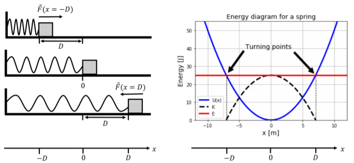
Figure $\PageIndex{1}$: Left: The block oscillates about the rest position of the spring, between $x = −D$ and $x = D$. Right: The energy diagram for the block. This diagram is for a spring with spring constant $k = 1 \text{N/m}$.

The energy diagram allows us to describe the motion of the object attached to the spring in terms of energy. A few things to note:

At $x=\pm D$, the potential energy is equal to $E$, so the kinetic energy is zero. The block is thus instantaneously at rest at those positions.
At $x=0$, the potential energy is zero, and the kinetic energy is maximal. This corresponds to where the block has the highest speed.
The kinetic energy of the block can never be negative¹, thus, the block cannot be located outside the range $[-D,+D]$, and we would say that the motion of the block is “bound”. The points between which the motion is bound are called “turning points”.

An analysis of the energy diagram tells us that the block is bound between the two turning points, which themselves are equidistant from the origin. When we initially compress the spring, we are “giving” the block “spring potential energy”. As the block starts to move, the potential energy of the block is converted into kinetic energy as it accelerates and then back into potential energy as it decelerates.

Exercise $\PageIndex{1}$

Calculate the positions of the turning points for the situation shown in Figure $\PageIndex{1}$. The total energy is $25\text{ J}$ and the spring constant is $k=\SI{1}{N/m}$.

Answer: $7.1\text{ m}$

By looking at only the potential energy function, without knowing that it is related to a spring, we can come to the same conclusions; namely that the motion is bound as long as the total mechanical energy is not infinite. We call the point $x=0$ a “stable equilibrium”, because it is a local minimum of the potential energy function. If the object is displaced from the equilibrium point, it will want to move back towards that point. This can also be understood in terms of the force associated with the potential energy function:

\[\begin{aligned} F = -\frac{d}{dx}U(x)\end{aligned}\]

The local minimum occurs where the derivative of the potential function is equal to zero. Thus, the equilibrium point is given by the condition that the force associated with the potential is zero ($x=0$ in the case of the potential energy from a spring). The equilibrium is a stable equilibrium because the force associated with the potential energy function ($F(x)=-kx$ for the spring) points towards the equilibrium point.

The potential energy function for an object with total mechanical energy, $E$, can be thought of as a little “roller coaster”, on which you place a marble and watch it “roll down” the potential energy function. You can think of placing a marble where $U(x)=E$ and releasing it. The marble would then roll down the potential energy function, just as an actual marble would roll down a real slope, mimicking the motion of the object along the $x$ axis. This is illustrated in Figure $\PageIndex{2}$ which shows an arbitrary potential energy function and a marble being placed at a location where the potential energy is equal to $E$.

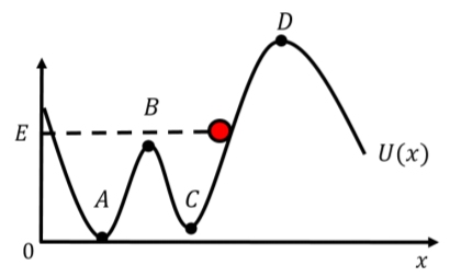
Figure $\PageIndex{2}$: Arbitrary potential energy function and illustration of visualizing a marble rolling down the function by placing the marble on the potential energy function at a point where $U(x) = E$.

The motion of the marble will be bound between the two points where the potential energy function is equal to $E$. When the marble is placed as shown, it will roll towards the left, just as if it were a real marble on a track. Since the potential energy is increasing as a function of $x$ at the point where we placed the marble, the force is in the negative $x$ direction (remember, the force is the negative of the derivative of the potential energy function). With the given energy, the marble would never be able to make it to point $D$, as it does not have enough energy to “climb up the hill”. It would roll down, through point $C$, up to point $B$, down to point $A$, and then turn around where $U(x)=E$ and return to where it started.

Locations $A$ and $C$ on the diagram are stable equilibria, because if a marble is placed in one of those locations and nudged slightly, it will come back to the equilibrium point (or oscillate about that point). Points $B$ and $D$ are “unstable equilibria”, because if the marble is placed there and nudged, it will not immediately come back to those points. Note that if the marble were placed at point $D$ and nudged towards the right, the motion of the marble would be unbound on the right, and it would keep going in that direction.

Now, say an object’s potential energy is described by the function in Figure $\PageIndex{2}$, and the object has total energy $E$. The object’s motion along the $x$ axis will be exactly the same as the projection of the marble’s motion on the $x$ axis.

Exercise $\PageIndex{2}$

A force, $F(x)$, acts on an object. The potential energy function, $U(x)$, associated with the force is given by $U(x)=a(x-6)^2(x-1)(x-3)+\SI{20}{J}$, where $a$ is a positive constant. $U(x)$ is plotted in Figure $\PageIndex{3}$. Use the “marble” method to determine the direction of the force at $x=5$. Confirm your answer by finding the value of the force , $F(x)$, at $x=5$.

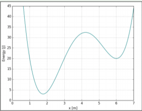
Figure $\PageIndex{3}$: A potential energy function $U(x)$. The $x$-axis represents the $x$ position and the $y$-axis represents the energy.

$F(x=5)=-10a$
$F(x=5)=10a$
$F(x=5)=20a$
$F(x=5)=-20a$

Answer

Footnotes

1. Remember, the kinetic energy is given by $K = \frac{1}{2}mv^{2}$. Since neither mass nor the value of $v^{2}$ can be negative, the kinetic energy of an object can never be negative.

Search

Text Color

Text Size

Margin Size

Font Type

Solution

Solution

Exercise \(\PageIndex{1}\)

Exercise \(\PageIndex{2}\)