9.16: Rolling Motion

Learning Objectives

• Describe the physics of rolling motion without slipping
• Explain how linear variables are related to angular variables for the case of rolling motion without slipping
• Find the linear and angular accelerations in rolling motion with and without slipping
• Calculate the static friction force associated with rolling motion without slipping
• Use energy conservation to analyze rolling motion

Rolling motion is that common combination of rotational and translational motion that we see everywhere, every day. Think about the different situations of wheels moving on a car along a highway, or wheels on a plane landing on a runway, or wheels on a robotic explorer on another planet. Understanding the forces and torques involved in rolling motion is a crucial factor in many different types of situations.

For analyzing rolling motion in this chapter, refer to Figure 10.5.4 in Fixed-Axis Rotation to find moments of inertia of some common geometrical objects. You may also find it useful in other calculations involving rotation.

Rolling Motion without Slipping

People have observed rolling motion without slipping ever since the invention of the wheel. For example, we can look at the interaction of a car’s tires and the surface of the road. If the driver depresses the accelerator to the floor, such that the tires spin without the car moving forward, there must be kinetic friction between the wheels and the surface of the road. If the driver depresses the accelerator slowly, causing the car to move forward, then the tires roll without slipping. It is surprising to most people that, in fact, the bottom of the wheel is at rest with respect to the ground, indicating there must be static friction between the tires and the road surface. In Figure \(\PageIndex{1}\), the bicycle is in motion with the rider staying upright. The tires have contact with the road surface, and, even though they are rolling, the bottoms of the tires deform slightly, do not slip, and are at rest with respect to the road surface for a measurable amount of time. There must be static friction between the tire and the road surface for this to be so.

Figure \(\PageIndex{1}\): (a) The bicycle moves forward, and its tires do not slip. The bottom of the slightly deformed tire is at rest with respect to the road surface for a measurable amount of time. (b) This image shows that the top of a rolling wheel appears blurred by its motion, but the bottom of the wheel is instantaneously at rest. (credit a: modification of work by Nelson Lourenço; credit b: modification of work by Colin Rose)

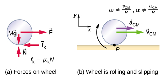
To analyze rolling without slipping, we first derive the linear variables of velocity and acceleration of the center of mass of the wheel in terms of the angular variables that describe the wheel’s motion. The situation is shown in Figure \(\PageIndex{2}\).

Figure \(\PageIndex{2}\): (a) A wheel is pulled across a horizontal surface by a force \(\vec{F}\). The force of static friction \(\vec{f}_{s}\), \(|\vec{f}_{s}|\) ≤ \(\mu_{s}\)N is large enough to keep it from slipping. (b) The linear velocity and acceleration vectors of the center of mass and the relevant expressions for \(\omega\) and \(\alpha\). Point P is at rest relative to the surface. (c) Relative to the center of mass (CM) frame, point P has linear velocity −R\(\omega \hat{i}\).

From Figure \(\PageIndex{2}\)(a), we see the force vectors involved in preventing the wheel from slipping. In (b), point P that touches the surface is at rest relative to the surface. Relative to the center of mass, point P has velocity −R\(\omega \hat{i}\), where R is the radius of the wheel and \(\omega\) is the wheel’s angular velocity about its axis. Since the wheel is rolling, the velocity of P with respect to the surface is its velocity with respect to the center of mass plus the velocity of the center of mass with respect to the surface:

\[\vec{v}_{P} = -R \omega \hat{i} + v_{CM} \hat{i} \ldotp\]

Since the velocity of P relative to the surface is zero, v_P = 0, this says that

\[v_{CM} = R \omega \ldotp \label{11.1}\]

Thus, the velocity of the wheel’s center of mass is its radius times the angular velocity about its axis. We show the correspondence of the linear variable on the left side of the equation with the angular variable on the right side of the equation. This is done below for the linear acceleration.

If we differentiate Equation \ref{11.1} on the left side of the equation, we obtain an expression for the linear acceleration of the center of mass. On the right side of the equation, R is a constant and since \(\alpha = \frac{d \omega}{dt}\), we have

\[a_{CM} = R \alpha \ldotp \label{11.2}\]

Furthermore, we can find the distance the wheel travels in terms of angular variables by referring to Figure \(\PageIndex{3}\). As the wheel rolls from point A to point B, its outer surface maps onto the ground by exactly the distance traveled, which is d_CM.

We see from Figure \(\PageIndex{3}\) that the length of the outer surface that maps onto the ground is the arc length R\(\theta\). Equating the two distances, we obtain

\[d_{CM} = R \theta \ldotp \label{11.3}\]

Figure \(\PageIndex{3}\): As the wheel rolls on the surface, the arc length R\(\theta\) from A to B maps onto the surface, corresponding to the distance d_CM that the center of mass has moved.

Example \(\PageIndex{1}\): Rolling Down an Inclined Plane

A solid cylinder rolls down an inclined plane without slipping, starting from rest. It has mass m and radius r. (a) What is its acceleration? (b) What condition must the coefficient of static friction \(\mu_{S}\) satisfy so the cylinder does not slip?

Strategy

Draw a sketch and free-body diagram, and choose a coordinate system. We put x in the direction down the plane and y upward perpendicular to the plane. Identify the forces involved. These are the normal force, the force of gravity, and the force due to friction. Write down Newton’s laws in the x- and y-directions, and Newton’s law for rotation, and then solve for the acceleration and force due to friction.

Solution

1. The free-body diagram and sketch are shown in Figure \(\PageIndex{4}\), including the normal force, components of the weight, and the static friction force. There is barely enough friction to keep the cylinder rolling without slipping. Since there is no slipping, the magnitude of the friction force is less than or equal to \(\mu_{S}\)N. Writing down Newton’s laws in the x- and y-directions, we have

\[\sum F_{x} = ma_{x};\; \sum F_{y} = ma_{y} \ldotp\]

Figure \(\PageIndex{4}\): A solid cylinder rolls down an inclined plane without slipping from rest. The coordinate system has x in the direction down the inclined plane and y perpendicular to the plane. The free-body diagram is shown with the normal force, the static friction force, and the components of the weight m\(\vec{g}\). Friction makes the cylinder roll down the plane rather than slip.

Substituting in from the free-body diagram

\[\begin{split} mg \sin \theta - f_{s} & = m(a_{CM}) x, \\ N - mg \cos \theta & = 0 \end{split}\]

we can then solve for the linear acceleration of the center of mass from these equations:

\[a_{CM} = g\sin \theta - \frac{f_s}{m} \ldotp\]

However, it is useful to express the linear acceleration in terms of the moment of inertia. For this, we write down Newton’s second law for rotation,

\[\sum \tau_{CM} = I_{CM} \alpha \ldotp\]

The torques are calculated about the axis through the center of mass of the cylinder. The only nonzero torque is provided by the friction force. We have

\[f_{s} r = I_{CM} \alpha \ldotp\]

Finally, the linear acceleration is related to the angular acceleration by

\[(a_{CM})_{x} = r \alpha \ldotp\]

These equations can be used to solve for a_CM, \(\alpha\), and f_S in terms of the moment of inertia, where we have dropped the x-subscript. We write a_CM in terms of the vertical component of gravity and the friction force, and make the following substitutions.

\[f_{S} = \frac{I_{CM} \alpha}{r} = \frac{I_{CM} a_{CM}}{r^{2}}\]

From this we obtain

\[\begin{split} a_{CM} & = g \sin \theta - \frac{I_{CM} a_{CM}}{mr^{2}}, \\ & = \frac{mg \sin \theta}{m + \left(\dfrac{I_{CM}}{r^{2}}\right)} \ldotp \end{split}\]

Note that this result is independent of the coefficient of static friction, \(\mu_{s}\).

Since we have a solid cylinder, from Figure 10.5.4, we have I_CM = \(\frac{mr^{2}}{2}\) and

\[a_{CM} = \frac{mg \sin \theta}{m + \left(\dfrac{mr^{2}}{2r^{2}}\right)} = \frac{2}{3} g \sin \theta \ldotp\]

Therefore, we have

\[\alpha = \frac{a_{CM}}{r} = \frac{2}{3r} g \sin \theta \ldotp\]

2. Because slipping does not occur, f_S ≤ \(\mu_{s}\)N. Solving for the friction force, $$f_{s} = I_{CM} \frac{\alpha}{r} = I_{CM} \frac{(a_{CM})}{r^{2}} = \left(\dfrac{I_{CM}}{r^{2}}\right) \left(\dfrac{mg \sin \theta}{m + \left(\dfrac{I_{CM}}{r^{2}}\right)}\right) = \frac{mg I_{CM} \sin \theta}{mr^{2} + I_{CM}} \ldotp$$Substituting this expression into the condition for no slipping, and noting that N = mg cos \(\theta\), we have $$\frac{mg I_{CM} \sin \theta}{mr^{2} + I_{CM}} \leq \mu_{s} mg \cos \theta$$or $$\mu_{s} \geq \frac{\tan \theta}{1 + \left(\dfrac{mr^{2}}{I_{CM}}\right)} \ldotp$$For the solid cylinder, this becomes $$\mu_{s} \geq \frac{\tan \theta}{1 + \left(\dfrac{2mr^{2}}{mr^{2}}\right)} = \frac{1}{3} \tan \theta \ldotp$$

Significance

1. The linear acceleration is linearly proportional to sin \(\theta\). Thus, the greater the angle of the incline, the greater the linear acceleration, as would be expected. The angular acceleration, however, is linearly proportional to sin \(\theta\) and inversely proportional to the radius of the cylinder. Thus, the larger the radius, the smaller the angular acceleration.
2. For no slipping to occur, the coefficient of static friction must be greater than or equal to \(\frac{1}{3}\)tan \(\theta\). Thus, the greater the angle of incline, the greater the coefficient of static friction must be to prevent the cylinder from slipping.

Exercise \(\PageIndex{2}\)

A hollow cylinder is on an incline at an angle of 60°. The coefficient of static friction on the surface is \(\mu_{s}\) = 0.6. (a) Does the cylinder roll without slipping? (b) Will a solid cylinder roll without slipping?

It is worthwhile to repeat the equation derived in this example for the acceleration of an object rolling without slipping:

\[a_{CM} = \frac{mg \sin \theta}{m + \left(\dfrac{I_{CM}}{r^{2}}\right)} \ldotp \label{11.4}\]

This is a very useful equation for solving problems involving rolling without slipping. Note that the acceleration is less than that for an object sliding down a frictionless plane with no rotation. The acceleration will also be different for two rotating cylinders with different rotational inertias.

Rolling Motion with Slipping

In the case of rolling motion with slipping, we must use the coefficient of kinetic friction, which gives rise to the kinetic friction force since static friction is not present. The situation is shown in Figure \(\PageIndex{5}\). In the case of slipping, v_CM − R\(\omega\) ≠ 0, because point P on the wheel is not at rest on the surface, and v_P ≠ 0. Thus, \(\omega\) ≠ \(\frac{v_{CM}}{R}\), \(\alpha \neq \frac{a_{CM}}{R}\).

Figure \(\PageIndex{5}\): (a) Kinetic friction arises between the wheel and the surface because the wheel is slipping. (b) The simple relationships between the linear and angular variables are no longer valid.

Example \(\PageIndex{2}\): Rolling Down an Inclined Plane with Slipping

A solid cylinder rolls down an inclined plane from rest and undergoes slipping (Figure \(\PageIndex{6}\)). It has mass m and radius r. (a) What is its linear acceleration? (b) What is its angular acceleration about an axis through the center of mass?

Strategy

Draw a sketch and free-body diagram showing the forces involved. The free-body diagram is similar to the no-slipping case except for the friction force, which is kinetic instead of static. Use Newton’s second law to solve for the acceleration in the x-direction. Use Newton’s second law of rotation to solve for the angular acceleration.

Solution

Figure \(\PageIndex{6}\): A solid cylinder rolls down an inclined plane from rest and undergoes slipping. The coordinate system has x in the direction down the inclined plane and y upward perpendicular to the plane. The free-body diagram shows the normal force, kinetic friction force, and the components of the weight m\(\vec{g}\).

The sum of the forces in the y-direction is zero, so the friction force is now f_k = \(\mu_{k}\)N = \(\mu_{k}\)mg cos \(\theta\). Newton’s second law in the x-direction becomes

\[\sum F_{x} = ma_{x}, \nonumber\]

\[mg \sin \theta - \mu_{k} mg \cos \theta = m(a_{CM})_{x}, \nonumber\]

or

\[(a_{CM})_{x} = g(\sin \theta - \mu_{k} \cos \theta) \ldotp \nonumber\]

The friction force provides the only torque about the axis through the center of mass, so Newton’s second law of rotation becomes

\[\sum \tau_{CM} = I_{CM} \alpha, \nonumber\]

\[f_{k} r = I_{CM} \alpha = \frac{1}{2} mr^{2} \alpha \ldotp \nonumber\]

Solving for \(\alpha\), we have

\[\alpha = \frac{2f_{k}}{mr} = \frac{2 \mu_{k} g \cos \theta}{r} \ldotp \nonumber\]

Significance

We write the linear and angular accelerations in terms of the coefficient of kinetic friction. The linear acceleration is the same as that found for an object sliding down an inclined plane with kinetic friction. The angular acceleration about the axis of rotation is linearly proportional to the normal force, which depends on the cosine of the angle of inclination. As \(\theta\) → 90°, this force goes to zero, and, thus, the angular acceleration goes to zero.

Conservation of Mechanical Energy in Rolling Motion

In the preceding chapter, we introduced rotational kinetic energy. Any rolling object carries rotational kinetic energy, as well as translational kinetic energy and potential energy if the system requires. Including the gravitational potential energy, the total mechanical energy of an object rolling is

\[E_{T} = \frac{1}{2} mv^{2}_{CM} + \frac{1}{2} I_{CM} \omega^{2} + mgh \ldotp\]

In the absence of any nonconservative forces that would take energy out of the system in the form of heat, the total energy of a rolling object without slipping is conserved and is constant throughout the motion. Examples where energy is not conserved are a rolling object that is slipping, production of heat as a result of kinetic friction, and a rolling object encountering air resistance.

You may ask why a rolling object that is not slipping conserves energy, since the static friction force is nonconservative. The answer can be found by referring back to Figure \(\PageIndex{2}\). Point P in contact with the surface is at rest with respect to the surface. Therefore, its infinitesimal displacement d\(\vec{r}\) with respect to the surface is zero, and the incremental work done by the static friction force is zero. We can apply energy conservation to our study of rolling motion to bring out some interesting results.

Example \(\PageIndex{3}\): Curiosity Rover

The Curiosity rover, shown in Figure \(\PageIndex{7}\), was deployed on Mars on August 6, 2012. The wheels of the rover have a radius of 25 cm. Suppose astronauts arrive on Mars in the year 2050 and find the now-inoperative Curiosity on the side of a basin. While they are dismantling the rover, an astronaut accidentally loses a grip on one of the wheels, which rolls without slipping down into the bottom of the basin 25 meters below. If the wheel has a mass of 5 kg, what is its velocity at the bottom of the basin?

Figure \(\PageIndex{7}\): The NASA Mars Science Laboratory rover Curiosity during testing on June 3, 2011. The location is inside the Spacecraft Assembly Facility at NASA’s Jet Propulsion Laboratory in Pasadena, California. (credit: NASA/JPL-Caltech)

Strategy

We use mechanical energy conservation to analyze the problem. At the top of the hill, the wheel is at rest and has only potential energy. At the bottom of the basin, the wheel has rotational and translational kinetic energy, which must be equal to the initial potential energy by energy conservation. Since the wheel is rolling without slipping, we use the relation v_CM = r\(\omega\) to relate the translational variables to the rotational variables in the energy conservation equation. We then solve for the velocity. From Figure \(\PageIndex{7}\), we see that a hollow cylinder is a good approximation for the wheel, so we can use this moment of inertia to simplify the calculation.

Solution

Energy at the top of the basin equals energy at the bottom:

\[mgh = \frac{1}{2} mv_{CM}^{2} + \frac{1}{2} I_{CM} \omega^{2} \ldotp \nonumber\]

The known quantities are I_CM = mr², r = 0.25 m, and h = 25.0 m.

We rewrite the energy conservation equation eliminating \(\omega\) by using \(\omega\) = v_CMr. We have

\[mgh = \frac{1}{2} mv_{CM}^{2} + \frac{1}{2} mr^{2} \frac{v_{CM}^{2}}{r^{2}} \nonumber\]

or

\[gh = \frac{1}{2} v_{CM}^{2} + \frac{1}{2} v_{CM}^{2} \Rightarrow v_{CM} = \sqrt{gh} \ldotp \nonumber\]

On Mars, the acceleration of gravity is 3.71 m/s², which gives the magnitude of the velocity at the bottom of the basin as

\[v_{CM} = \sqrt{(3.71\; m/s^{2})(25.0\; m)} = 9.63\; m/s \ldotp \nonumber\]

Significance

This is a fairly accurate result considering that Mars has very little atmosphere, and the loss of energy due to air resistance would be minimal. The result also assumes that the terrain is smooth, such that the wheel wouldn’t encounter rocks and bumps along the way.

Also, in this example, the kinetic energy, or energy of motion, is equally shared between linear and rotational motion. If we look at the moments of inertia in Figure 10.5.4, we see that the hollow cylinder has the largest moment of inertia for a given radius and mass. If the wheels of the rover were solid and approximated by solid cylinders, for example, there would be more kinetic energy in linear motion than in rotational motion. This would give the wheel a larger linear velocity than the hollow cylinder approximation. Thus, the solid cylinder would reach the bottom of the basin faster than the hollow cylinder.

Rolling Without Slipping and Pulleys

A very large number of the mechanical energy conservation problems we will do involve the relation we discussed previously that relates rotational motion to linear motion. Specifically we will apply this to what is referred to as rolling without slipping, or perfect rolling. There are two reasons this is an important condition to understand:

• When two surfaces slip across each other, thermal energy is the result. So when an object rolls without slipping, there may be static friction present, but there is no kinetic friction, which means that no thermal energy is produced and mechanical energy is conserved.
• When a round object rolls perfectly, the distance it travels in a straight line is directly related to the angle through which it rotates.

We’ll keep the first observation in mind for later, but right now let’s focus on the second condition:

Figure \(\PageIndex{8}\) – Perfect Rolling

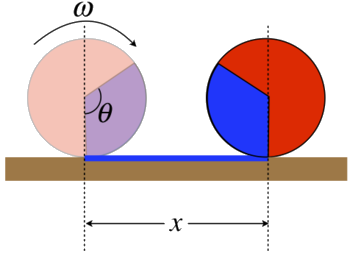
The linear distance traveled equals the arclength of the shaded region if the wheel is rolling without slipping, so we have:

\[ x = arclength = R\theta \;\;\; \Rightarrow \;\;\; v = \dfrac{dx}{dt} = R\dfrac{d\theta}{dt} = R\omega \]Imagine now that instead of this being a wheel, it is a spool that is unwinding. Then the blue line represents string that is coming off the spool. We can therefore conclude that the relation \(v = R\omega\) also applies to the linear speed of a rope that is either unraveling from a rotating spool or passing over a turning pulley.

Total Kinetic Energy as a Sum of Linear and Rotational

It’s time we considered the case of an object whose center of mass is moving while it rotates. Let’s start with a simple case of two rocks of different masses attached by a string:

Figure \(\PageIndex{9}\) – Unbalanced Dumbell Spinning as It Moves

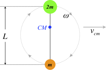
This system is rotating as its center of mass moves in a straight line (assume there is no gravity present). We are given its rotational speed \(\omega\) and the velocity of its center of mass, and wish to answer the question, "How much kinetic energy does this system possess at the moment depicted in the diagram?"

We could easily answer this question if we knew the speeds of the two rocks, but we are not given those numbers. We have to extract them from what is given, and this requires some thought. We know three things that get us to this answer:

• The velocity of a rock relative to us equals its velocity relative to the center of mass, plus the velocity of the center of mass.
• The center of mass lies at the point two-thirds of the distance from \(m\) to \(2m\).
• The rotational velocities of both rocks are the same, but the linear velocities relative to the center of mass depend upon their distances from the center of mass according to the usual \(v=r\omega\).

Let us label the bottom rock as #1, and the top rock as #2. Putting the first and third conditions together first gives us:

\[v_1=v_{cm}-r_1\omega \;\;\;\;\;\;\;\;\;\; v_2=v_{cm}+r_2\omega \]

The sign of the second term in each equation is determined by whether the rotational motion adds to or takes away from the linear motion of the center of mass. Next we invoke the second condition. The fact that the center of mass is two-thirds of the distance from \(m\) to \(2m\) means:

\[r_1 = \frac{2}{3}L \;\;\;\;\;\;\;\;\;\; r_2 = \frac{1}{3}L \]

Putting all of the above into the kinetic energy of the system gives an expression for the total kinetic energy in terms of the values given. Collecting terms proportional to the squares of center of mass velocity and angular velocity gives:

\[ \begin{array}{l} KE_{tot} & = KE_1+KE_2 \\ & = \frac{1}{2}mv_1^2 + \frac{1}{2}\left(2m\right)v_2^2 \\ & = \frac{1}{2}m\left[v_{cm}-r_1\omega\right]^2 + \frac{1}{2}\left(2m\right)\left[v_{cm}+r_2\omega\right]^2 \\ & = \frac{1}{2}m\left[v_{cm}-\left( \frac{2}{3}L \right)\omega\right]^2 + \frac{1}{2}\left(2m\right)\left[v_{cm}+\left( \frac{1}{3}L\right)\omega\right]^2 \\ & = \frac{1}{2} \left(3m\right)v_{cm}^2 + \frac{1}{2} \left(\frac{2}{3}mL^2\right)\omega^2 \end{array} \]

The \(3m\) in the first term is the total mass of the system, so the first term is the kinetic energy of system if was not spinning. That means that the second term is the amount of kinetic energy added to the system by virtue of its spinning. The part of the second term in parentheses looks suspiciously like a rotational inertia, and in fact it equals the rotational inertia of the system about its center of mass:

\[ I_{cm} = m_1r_1^2 + m_2r_2^2 = \left(m\right)\left(\frac{2}{3}L\right)^2 + \left(2m\right)\left(\frac{1}{3}L\right)^2 = \frac{2}{3}mL^2 \]

This turns out to be a completely general rule for the kinetic energy of an object that is rotating as its center of mass moves:

\[ KE_{tot} = KE_{lin} + KE_{rot} = \frac{1}{2}mv_{cm}^2 + \frac{1}{2}I_{cm}\omega^2 \]

Exercise

Show the same result for two general point masses \(m_1\) and \(m_2\) separated by an unknown distance (call their distances from the center of mass \(r_1\) and \(r_2\)), this time using the moment in time when \(m_1\) is directly in front of \(m_2\) (i.e. the line joining them is horizontal).

Solution

At the moment when the two masses form a horizontal line, their linear motions due to rotation are perpendicular to the center of mass motion. Determining their total speeds is therefore a simple application of the Pythagorean theorem, and the result follows surprisingly quickly:

\[ \begin{array}{l} v_1^2 = v_{cm}^2 + \left(r_1\omega\right)^2 \\ v_2^2 = v_{cm}^2 + \left(r_2 \omega \right)^2 \end{array} \nonumber\]

Now plug this into the kinetic energy for the system as the sum of the kinetic energies of the two masses:

\[ \begin{array}{l} KE_{tot} & = \frac{1}{2} m_1 v_1^2 + \frac{1}{2} m_2 v_2^2 \\ & = \frac{1}{2} m_1 \left(v_cm^2 + r_1^2 \omega^2 \right) + \frac{1}{2} m_2 \left(v_{cm}^2 + r_2^2 \omega^2 \right) \\ & = \frac{1}{2} \left(m_1 + m_2 \right) v_{cm}^2 + \frac{1}{2} \left(m_1r_1^2 + m_2 r_2^2 \right) \omega^2 \end{array} \nonumber \]

While the above equation is generally true for any object, if the object is rotating about a fixed point, the expression for total KE can be simpler to write. Specifically, it is what we have written before, in terms of the rotational inertia about the fixed point:

\[ KE_{tot} = \frac{1}{2}I_{fixed \; point}\omega^2 \]

Assuming the fixed point is not the center of mass (or the assertion is proved trivially), then let’s call the distance from the center of mass to the fixed point “\(d\).” The center of mass is following a circular path of radius \(d\) around the fixed point, which means we can relate the linear velocity of the center of mass to its angular velocity around the fixed point:

\[ v_{cm} = \omega d \]

Putting this into our center-of-mass energy equation gives:

\[ {KE}_{tot} = \frac{1}{2}mv^2_{cm} + \frac{1}{2}I_{cm}\omega^2 = \frac{1}{2}m \left(\omega d \right)^2 + \frac{1}{2}I_{cm} \omega^2 = \frac{1}{2} \underbrace{ \left( md^2 + I_{cm} \right) }_{I_{fixed \; point}}\omega^2 \]

Where in the final step we employed the parallel-axis theorem.

Analyze This

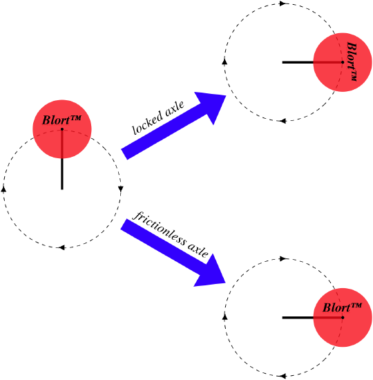
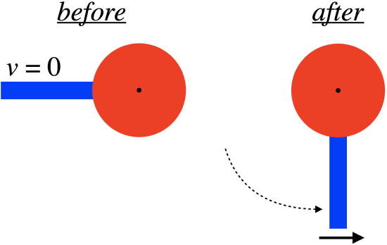
The Blort Corporation makes a special widget that consists of a uniform disk pivoted around an axle at the end of a rod of negligible mass, which in turn rotates about its other end. This widget has two settings: It can be set in the "locked" position so that the disk does not rotate around its axle, or the "free" position so that the disk rotates frictionlessly about the axle. The difference these settings have on the motion of the disk as the rod rotates is depicted in the figure below.

Analysis

If we call the mass of the disk \(M\), the radius of the disk \(R\), the length of the rod \(L\), and the rate at which the rod is rotating \(\omega\), we can compute the kinetic energies of these two settings. In the case of the free setting, the disk is simply moving in a circle without rotating, so it has only the linear component of kinetic energy:

\[{KE}_{free}=\frac{1}{2}mv_{cm}^2+0=\frac{1}{2}M\left(L\omega\right)^2=\frac{1}{2}ML^2\omega^2\nonumber\]

For the locked axle case, we can find the energy two ways. The first is to treat the rod + disk as a single rigid object (which of course it is), with a fixed point for the rotation. The rod has no mass, but we can find the moment of inertia of this rigid object using the parallel-axis theorem:

\[{KE}_{locked}=\frac{1}{2}I_{fixed}\omega^2=\frac{1}{2}\left(\frac{1}{2}MR^2+ML^2\right)\omega^2=\frac{1}{4}M\left(R^2+2L^2\right)\omega^2\nonumber\]

Alternatively, we can use the linear + rotational form of kinetic energy, and the same result as this is attained. To use this method, one needs to figure out the rotational speed of the disk. It's not immediately obvious that it is the same as the rotational speed of the rod, so consider this: In one full revolution of the rod with the locked axle, the disk also makes exactly one full revolution. So the rotational rate of the disk is also \(\omega\).

What is clear about this result is that for the same rotational speed for the rod, a different amount of kinetic energy is in the system for the two settings. The way we put energy into a system is to do work on it, so it appears that to achieve the same rotational speed of the rod, more work is required for the locked setting than for the free setting.

Mechanical Energy Conservation with Perfect Rolling

Let's put together what we have concluded so far in this section. We begin by noting that two cylinders with equal masses do not possess the same rotational inertia about their central axes if one is hollow and the other is solid. Now imagine rolling both of these cylinders (without slipping) down an inclined plane. Can you guess which one would reach the bottom of the incline with the greater speed? The main point to be made here is that the energy that comes from gravitational PE goes into KE, but now the KE has two different forms: linear and rotational. The linear and angular speeds are directly related through the "no slipping" condition, so the energy will convert into the two forms of kinetic energy in a fixed ratio. We will soon see how the rotational inertia affects the ratio, but it seems clear that the hollow cylinder puts more of its energy into rotation (for the same velocity) than the solid cylinder. This would seem to indicate that the hollow will have the same kinetic energy as the solid cylinder only if it is turning (and therefore moving) more slowly.

It's easy to trick oneself in such situations, so let's solve the math carefully to be sure.

Figure \(\PageIndex{10}\) – Comparing Hollow and Solid Cylinder Rolling Dynamics

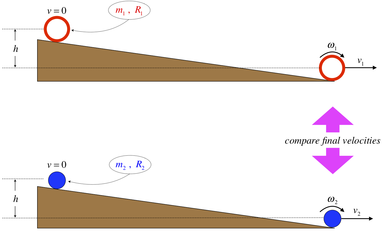
We will work both problems in parallel, to make the difference more evident. Start with mechanical energy conservation from the top of the plane to the bottom. We can invoke this because without slipping there is no rubbing, which means no mechanical energy is converted to thermal energy.

\[ \Delta KE + \Delta PE_{grav} =0 \;\;\; \Rightarrow \;\;\; KE_o + PE_o = KE_f + PE_f \]

If we choose the zero point of potential energy to be the bottom of the incline, the initial and final potential energies in both cases are \(mgh\) and zero, respectively. The initial kinetic energy is zero in both cases, and the final kinetic energy is the sum of the linear and rotational kinetic energies (Equation 5.3.6):

\[ \begin{array}{rlll} & hollow\;cylinder & & solid\;cylinder \\ \\ energy\:conservation: & m_1gh = \frac{1}{2}m_1v_{1f}^2 + \frac{1}{2}I_1\omega_{1f}^2 & & m_2gh = \frac{1}{2}m_2v_{2f}^2 + \frac{1}{2}I_2\omega_{2f}^2 \\ perfect\;rolling \left(v=R\omega\right): & m_1gh = \frac{1}{2}m_1v_{1f}^2 + \frac{1}{2}I_1\left(\dfrac{v_{1f}}{R_1}\right)^2 & & m_2gh = \frac{1}{2}m_2v_{2f}^2 + \frac{1}{2}I_2\left(\dfrac{v_{2f}}{R_2}\right)^2 \\ rotational\;inertia\;of\;cylinders: & m_1gh = \frac{1}{2}m_1v_{1f}^2 + \frac{1}{2}\left(m_1R_1^2\right)\left(\dfrac{v_{1f}}{R_1}\right)^2 & & m_1gh = \frac{1}{2}m_2v_{2f}^2 + \frac{1}{2}\left(\frac{1}{2}m_2R_2^2\right)\left(\dfrac{v_{2f}}{R_2}\right)^2 \\ algebra: & v_{1f} = \sqrt{gh} & & v_{2f} = \sqrt{\dfrac{4gh}{3}} \end{array}\]

So in fact the solid cylinder is moving faster than the hollow one, as we predicted. What is especially interesting is that with the perfect rolling condition in place, the masses and radii of the cylinders are irrelevant! We are used to final speeds of objects accelerated by gravity being independent of the mass, but here we see that when we impose perfect rolling, the radius also plays no role, but the distribution of the mass within the cylinder is all that matters.

Alert

As we are discussing mechanical energy conservation again, it is a good time to remind ourselves that our conclusions only tell us how to compare speeds before and after – what goes on between these two moments and direction of motion are lost bits of information. This is as true now that rotation is involved as it was when it wasn't. For example, if we were to race the two cylinders down identical ramps, then naturally the solid cylinder would get to the bottom first, since they both start at rest and accelerate at constant rates. The object with the faster final speed must have taken less time to get to the bottom because it had a greater average velocity. The math shown above doesn't take into account the paths the two cylinders take, so if the ramps are not identical (but still result in the same height change), the conclusion about speeds at the bottom is the same as before, but the winner of the race may not be the solid cylinder!

Analyze This

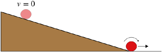
A solid uniform sphere starts from rest and rolls down a flat ramp without slipping. 

Analysis

Calling the height that the sphere descends \(h\), we can compute its final speed using mechanical energy conservation. Following the usual method of including both the linear and rotational kinetic energy, we get:

\[{KE}_{before}+U_{before} = {KE}_{after}+U_{after} \;\;\;\Rightarrow\;\;\; mgh+0=\left(\frac{1}{2}mv_{cm}^2+\frac{1}{2}I\omega^2\right)+0\nonumber\]

The moment of inertia of a solid sphere is \(\frac{2}{5}mR^2\), so putting this in and noting that perfect rolling means \(v=R\omega\), we have:

\[mgh=\frac{1}{2}mv^2+\frac{1}{2}\left(\frac{2}{5}mR^2\right)\left(\frac{v}{R}\right)^2=\frac{7}{10}mv^2\;\;\;\Rightarrow\;\;\;v=\sqrt{\frac{10}{7}gh}\nonumber\]

Another thing we can note in the analysis is that the free-body diagram of the sphere never changes during its time on the ramp, so its acceleration must remain constant. With a constant linear acceleration, and the starting and ending speeds, we can possibly extract more information from kinematics equations.

Analyze This

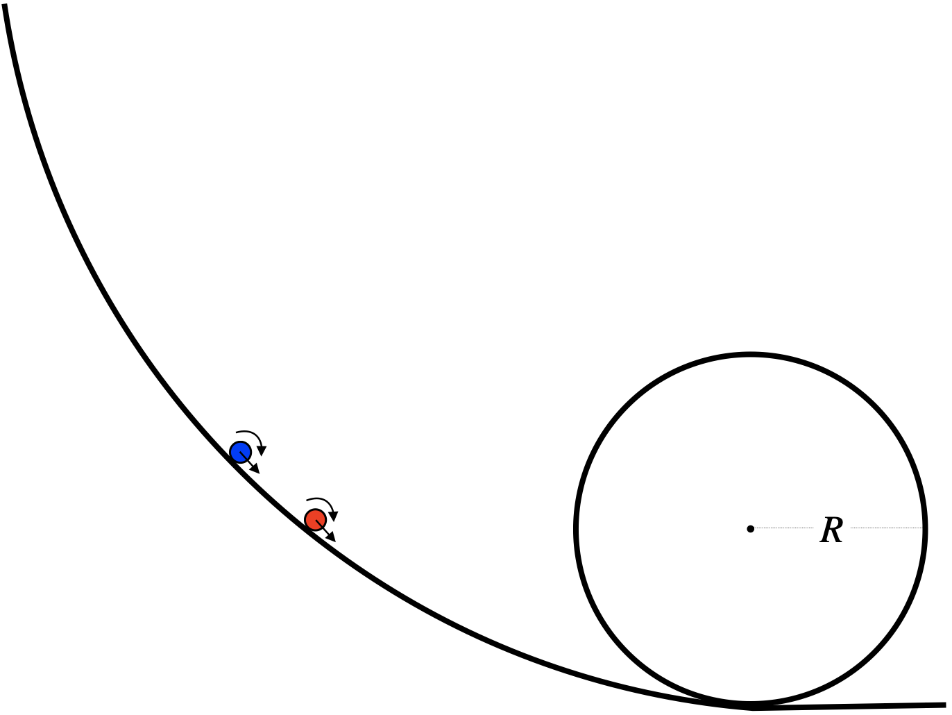
A solid and a hollow sphere roll without slipping simultaneously (one behind the other) down a ramp and around a loop-de-loop. The radii of the spheres are negligible compared to the radius of the loop.

Analysis

The rolling-without-slipping condition relates the linear speeds of the spheres to their rotational speeds according to \(v=R\omega\). This results in an amount of kinetic energy for each sphere that is different for a given linear speed, because they have different moments of inertia:

\[KE_{solid}=\frac{1}{2}mv^2+\frac{1}{2}I\omega^2=\frac{1}{2}mv^2+\frac{1}{2}\left(\frac{2}{5}mR^2\right)\omega^2=\frac{7}{10}mv^2\nonumber\]

\[KE_{hollow}=\frac{1}{2}mv^2+\frac{1}{2}I\omega^2=\frac{1}{2}mv^2+\frac{1}{2}\left(\frac{2}{3}mR^2\right)\omega^2=\frac{5}{6}mv^2\nonumber\]

The typical thing to think about in cases where a loop-de-loop is involved whether the object has enough speed to make it around. With the spheres having very small radii, they are essentially moving in a circular path with a radius equal to that of the loop as they go around. In order to make it around, they have to be barely moving fast enough that the gravitational force is providing all the pull necessary to keep them going in a circle at the top of the loop – any faster and there would be normal force from the loop, and any slower and the sphere would fall off the loop. This condition therefore requires that the sphere has speed of:

\[\frac{v^2}{R}=g\;\;\;\Rightarrow\;\;\;v=\sqrt{gR}\nonumber\]

Massive Spools

Another example that falls into this same category of mechanical energy conservation with perfect rolling is a falling mass unwinding a massive spool. Let's assume the spool is frictionless and is a uniform disk, and determine the speed of the falling block after it has dropped a known distance. We are also assuming – as always – that the string is massless, but we should also point out that it is very thin, so that its departure from the spool does not reduce the radius of the spool.

Figure \(\PageIndex{11}\) – Falling Block Unwinds Spool

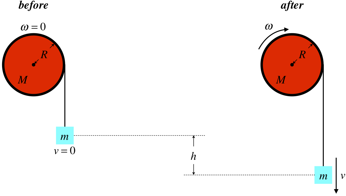
Once again, we can solve this using mechanical energy conservation, as there are no non-conservative forces present. What is new here is that some of the potential energy lost by the block as it drops goes into the rotational kinetic energy of the spool. The math is strikingly similar to the rolling cylinder case above:

\[ \begin{array}{rl} energy\:conservation: & mgh = \frac{1}{2} mv^2 + \frac{1}{2} I \omega^2 \\ perfect\;rolling \left( v=R \omega \right): & mgh = \frac{1}{2}mv^2 + \frac{1}{2} I \left( \dfrac{v}{R} \right)^2 \\ rotational\;inertia\;of\;spool: & mgh = \frac{1}{2}mv^2 + \frac{1}{2} \left( \frac{1}{2} MR^2 \right) \left(\dfrac{v}{R} \right)^2 \\ algebra: & v = \sqrt{ \dfrac{4mgh}{2m+M} } \end{array} \]

Analyze This

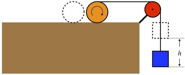
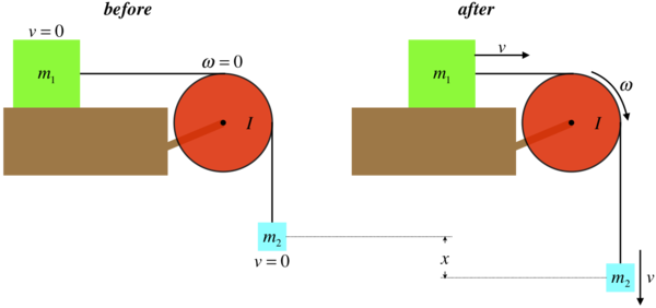
One end of a massless rope is wound around a uniform solid cylinder, while the other end passes over a massless, frictionless pulley and is attached to a hanging block, as in the diagram below. The block is released from rest, pulling the cylinder along the horizontal surface such that it rolls without slipping.

Analysis

The amount that the block falls equals the distance traveled by the cylinder plus the length of rope that unwinds from it. Since the cylinder rolls without slipping, the amount that unwinds is also equal to the distance it travels, so the sum of the distance traveled by the cylinder and the rope unwound is just double the distance that the cylinder travels. Therefore, the speed of the block is at all times twice the linear speed of the cylinder.

With no non-conservative forces present, the mechanical energy of the system is conserved, so subscripting the masses and velocities with 'b' for block, and 'c' for cylinder, we get:

\[ m_bgh = \frac{1}{2}m_bv_b^2 + \frac{1}{2}m_cv_c^2 + \frac{1}{2}I\omega^2 \nonumber \]

We know the rotational inertia of the cylinder in terms of its mass and radius, that the block moves twice as fast as the cylinder, and that the cylinder rolls without slipping. Putting all of these constraints into the equation above gives us our answer:

\[ \left. \begin{array}{l} I = \frac{1}{2}m_cR^2 \\ v_b = 2v_c \\ R\omega = v_c \end{array} \right\} \;\;\; \Rightarrow \;\;\; m_bgh = \frac{1}{2}m_b \left( 2v_c \right)^2 + \frac{1}{2}m_cv_c^2 + \frac{1}{2}\left( \frac{1}{2} m_cR^2 \right) \omega^2 =\frac{1}{2}\left(4m_b+\frac{3}{2}m_c\right)v_c^2\nonumber \]

Solving for the speed of the cylinder (and the speed of the block is twice this much):

\[v_c=\sqrt{\frac{4m_b}{8m_b+3m_c}gh}\nonumber\]

The linear acceleration of the block and spool are constant, so knowing the final velocity allows us to use kinematics equations if we are given additional information.

Massive Pulleys

The result for this example may remind you of an assumption we made long ago regarding pulleys. We have always assumed that they were frictionless and massless. We said that the result of these assumptions was that the tension for the rope was the same everywhere (namely on both sides of the pulley). We are now equipped to look at what happens if the pulley has mass. We'll do so with a simple model physical system. In Figure 5.3.5, the hanging block accelerates as it falls, linearly accelerating the block on the frictionless horizontal surface and rotationally accelerating the pulley in the process.

Figure \(\PageIndex{12}\) – Effect of a Massive Pulley on Rope Tension

We are interested in comparing the tension force by the rope on both sides of this pulley, so let's use the work-energy theorem, which takes into account the forces. Treating each block as a separate system, on which the tension in each end of the rope performs work (and gravity does work on block #2 as well), and noting that both move at the same speed at all times, we have:

\[ \begin{array}{lcr} W_1 = \Delta KE_1 & \Rightarrow & T_1 \cdot x = \frac{1}{2} m_1v^2 \\ W_2 = \Delta KE_2 & \Rightarrow & \left(m_2g-T_2\right) \cdot x = \frac{1}{2} m_2v^2 \end{array} \]

Let's compare the two tensions by computing the difference:

\[ \left(T_1 - T_2\right) \cdot x = \underbrace{\frac{1}{2}m_1v^2 + \frac{1}{2}m_2v^2}_{\Delta KE_{blocks}} \; \underbrace{- \; m_2gx}_{\Delta PE_{grav}} \]

For the tensions to be equal, all of the gravitational potential energy lost by the falling block must go into the two blocks. But we now know that a massive pulley will have kinetic energy. Let's add the pulley's increase in kinetic energy to both sides of the equation, and invoke mechanical energy conservation:

\[ \left(T_1 - T_2\right) \cdot x + \left[\frac{1}{2}I\omega^2 \right]= \Delta KE_{blocks} + \left[\Delta KE_{pulley}\right] + \Delta PE_{grav} = 0 \;\;\; \Rightarrow \;\;\; T_1 - T_2 = \dfrac{\frac{1}{2}I\omega^2}{x} \]

The tensions can only be equal when the rotational inertia of the pulley is zero, which means it must be massless.

Analyze This

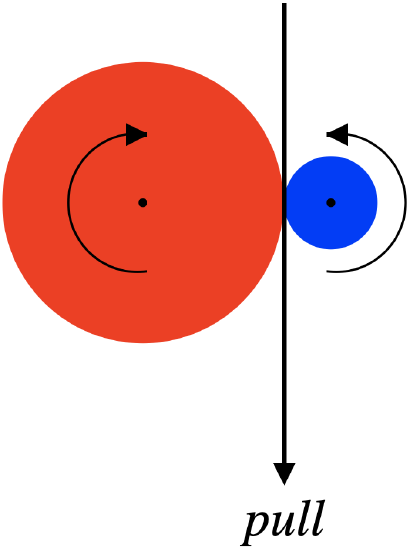
Two disks are cut out of the same material, as shown in the diagram below. They are pivoted around stationary axles such that the two disks lie in the vertical plane, with their outer rims pinching a massless rope between them. The rope is pulled downward, causing both disks to turn without the rope slipping.

Analysis

Let's call the radii of the large disk \(R\) and of the small disk \(r\). We are given that they are made of the same uniform material, so their masses are proportional to their areas, which means their masses have the following ratio:

\[\frac{M}{m}=\frac{\pi R^2}{\pi r^2} = \left(\frac{R}{r}\right)^2\nonumber\]

The ratio of their moments of inertia can therefore also be written in terms of their radii:

\[\frac{I_{large}}{I_{small}}=\dfrac{\frac{1}{2}MR^2}{\frac{1}{2}mr^2}=\left(\frac{M}{m}\right)\left(\frac{R^2}{r^2}\right)=\left(\frac{R}{r}\right)^4\nonumber\]

When the rope is pulled, the disks don't slip, which means that their edges are moving at the same linear speed. Because of the perfect rolling condition, this means that they do not rotate at the same angular speed, and the ratios of these speeds is also expressible in terms of the ratio of radii:

\[v_{rope}=R\omega_{large}=r\omega_{small}\;\;\;\Rightarrow\;\;\;\frac{\omega_{large}}{\omega_{small}}=\frac{r}{R}\nonumber\]

Digression: Energy Storage

One of the big issues today with green energy like solar and wind-generated electricity, is storage. The advantage to fossil fuel production of electricity is that we can produce it whenever we like, but for solar and wind power, we are at the mercy of when the sun shines or the wind blows. So storing the energy generated from these green sources is of paramount importance. Batteries are coming along, but they have their own environmental issues (lithium mining, waste when they degrade, etc.), so other means of storage are sought.

There are many ideas that have been put forth, such as using spare electricity to pump water above a dam so that it can be released when needed; pressurizing tanks of air with spare electricity, then allowing the pressurized air to drive a generator later; and using spare electricity to desalinate water, followed by using the osmotic pressure between the new fresh water and the salty water to drive a generator. But possibly the best idea (which has been around a long time) is to simply store the energy in the form of kinetic energy – spin a flywheel. A flywheel is just a disk created for the sole purpose of spinning so that it holds kinetic energy until it can be used later. The idea is for the spare electricity to get this thing spinning (with as little friction as possible), so that later when we need the energy back, the flywheel can be connected to a generator and the kinetic energy can be converted back into electrical energy. The beauty of this idea is in its simplicity – it is inexpensive and scalable. And reducing the friction to a very low value is something we can do quite well with today’s technology (think maglev and evacuated chambers). In order to be as efficient with our use of space as possible, and so that we don’t reach rotational speeds that are insanely high, we will of course want flywheels with very large rotational inertias.

Swinging Around Fixed Points

There is one other common physical situation involving mechanical energy conservation and rotation that needs to be addressed. If a rigid extended object is pivoted around a fixed point that is not the center of mass, and it is allowed to swing around that pivot under the influence of gravity, then how do we use mechanical energy conservation to describe its motion? Specifically, as the object swings, some points of the object may move upward (increasing gravitational potential energy), while others may swing downward (decreasing gravitational potential energy). How can we deal with the overall change in gravitational potential energy in such a case?

The answer will likely be unsurprising. Write the change of potential energy of the whole object as the sum of the potential energies of each tiny mass that makes up the object, and the result follows immediately:

\[ \begin{array}{l} \Delta U\left(whole\;object\right) & = \Delta U_1 + \Delta U_2 + \dots \\ & = m_1g\Delta y_1 + m_2g\Delta y_2 + \dots \\ & = \dfrac{Mg}{M}\left(m_1\Delta y_1 + m_2\Delta y_2 + \dots\right) \\ & = Mg\dfrac{m_1\Delta y_1 + m_2\Delta y_2 + \dots}{M}=Mg\Delta y_{cm} \end{array}\]

where \(M = m_1 + m_2\ + \dots\) is the mass of the whole object and \(\Delta y_{cm}\) is the change in height of the center of mass of the object.

Analyze This

One end of a uniform metal thin rod is welded to the outer edge of a metal disk. The masses of these two objects are the same, and the length of the rod is equal to the diameter of the disk. The disk is suspended on a frictionless axle positioned at its center, and the rod is released from rest from a horizontal orientation and allowed to swing down to the vertical position.

Analysis

This system experiences a loss of gravitational potential energy during this swing, which can be measured in two different ways. First, we can just use the method above, where we find the center of mass of the whole system before and after, and use its full mass and that drop. In this case, with the length of rod equaling the diameter of the disk, the center of mass of the rod is a distance \(R\) (the radius of the disk) from the weld point. The center of mass of the disk is also this distance from the weld point, and since the masses of the disk and rod are equal, the weld point must be its center of mass. This point drops a distance of \(R\), so the loss of potential energy (with \(m\) defined as the mass of each object) is just:

\[\Delta U =-2mgR\nonumber\]

A second way to do this, which may be a bit simpler to use, is to note that the center of mass of the rod drops a distance \(2R\), while the center of mass of the disk does not change at all, giving the same potential energy change:

\[\Delta U = \Delta U_{rod} + \Delta U_{disk} = -mg\left(2R\right) + 0=-2mgR\nonumber\]

This potential energy becomes kinetic energy. The object swings around a fixed point, so we can compute the moment of inertia about the fixed point and use the usual formula. To get this moment of inertia, we'll need the additivity of moments of inertia and the parallel axis theorem. The disk about the axle has a well-known moment of inertia. To get the contribution of the rod, we use its moment of inertia about its center of mass, and displace it a distance of \(2R\) using the parallel axis theorem:

\[I_{tot}=I_{disk}+I_{rod}=\frac{1}{2}mR^2+\left[\frac{1}{12}m(2R)^2+m\left(2R\right)^2\right]=\frac{29}{6}mR^2\nonumber\]

Putting this into the energy conservation equation and solving for the angular speed of the swing at the bottom of the arc gives:

\[{KE}_f=-\Delta U \;\;\;\Rightarrow\;\;\; \frac{1}{2}\left(\frac{29}{6}mR^2\right)\omega^2=2mgR\;\;\;\Rightarrow\;\;\; \omega=\sqrt{\frac{24g}{29R}}\nonumber\]