10.5: Forced Oscillations
- Page ID
- 68845
\( \newcommand{\vecs}[1]{\overset { \scriptstyle \rightharpoonup} {\mathbf{#1}} } \)
\( \newcommand{\vecd}[1]{\overset{-\!-\!\rightharpoonup}{\vphantom{a}\smash {#1}}} \)
\( \newcommand{\dsum}{\displaystyle\sum\limits} \)
\( \newcommand{\dint}{\displaystyle\int\limits} \)
\( \newcommand{\dlim}{\displaystyle\lim\limits} \)
\( \newcommand{\id}{\mathrm{id}}\) \( \newcommand{\Span}{\mathrm{span}}\)
( \newcommand{\kernel}{\mathrm{null}\,}\) \( \newcommand{\range}{\mathrm{range}\,}\)
\( \newcommand{\RealPart}{\mathrm{Re}}\) \( \newcommand{\ImaginaryPart}{\mathrm{Im}}\)
\( \newcommand{\Argument}{\mathrm{Arg}}\) \( \newcommand{\norm}[1]{\| #1 \|}\)
\( \newcommand{\inner}[2]{\langle #1, #2 \rangle}\)
\( \newcommand{\Span}{\mathrm{span}}\)
\( \newcommand{\id}{\mathrm{id}}\)
\( \newcommand{\Span}{\mathrm{span}}\)
\( \newcommand{\kernel}{\mathrm{null}\,}\)
\( \newcommand{\range}{\mathrm{range}\,}\)
\( \newcommand{\RealPart}{\mathrm{Re}}\)
\( \newcommand{\ImaginaryPart}{\mathrm{Im}}\)
\( \newcommand{\Argument}{\mathrm{Arg}}\)
\( \newcommand{\norm}[1]{\| #1 \|}\)
\( \newcommand{\inner}[2]{\langle #1, #2 \rangle}\)
\( \newcommand{\Span}{\mathrm{span}}\) \( \newcommand{\AA}{\unicode[.8,0]{x212B}}\)
\( \newcommand{\vectorA}[1]{\vec{#1}} % arrow\)
\( \newcommand{\vectorAt}[1]{\vec{\text{#1}}} % arrow\)
\( \newcommand{\vectorB}[1]{\overset { \scriptstyle \rightharpoonup} {\mathbf{#1}} } \)
\( \newcommand{\vectorC}[1]{\textbf{#1}} \)
\( \newcommand{\vectorD}[1]{\overrightarrow{#1}} \)
\( \newcommand{\vectorDt}[1]{\overrightarrow{\text{#1}}} \)
\( \newcommand{\vectE}[1]{\overset{-\!-\!\rightharpoonup}{\vphantom{a}\smash{\mathbf {#1}}}} \)
\( \newcommand{\vecs}[1]{\overset { \scriptstyle \rightharpoonup} {\mathbf{#1}} } \)
\(\newcommand{\longvect}{\overrightarrow}\)
\( \newcommand{\vecd}[1]{\overset{-\!-\!\rightharpoonup}{\vphantom{a}\smash {#1}}} \)
\(\newcommand{\avec}{\mathbf a}\) \(\newcommand{\bvec}{\mathbf b}\) \(\newcommand{\cvec}{\mathbf c}\) \(\newcommand{\dvec}{\mathbf d}\) \(\newcommand{\dtil}{\widetilde{\mathbf d}}\) \(\newcommand{\evec}{\mathbf e}\) \(\newcommand{\fvec}{\mathbf f}\) \(\newcommand{\nvec}{\mathbf n}\) \(\newcommand{\pvec}{\mathbf p}\) \(\newcommand{\qvec}{\mathbf q}\) \(\newcommand{\svec}{\mathbf s}\) \(\newcommand{\tvec}{\mathbf t}\) \(\newcommand{\uvec}{\mathbf u}\) \(\newcommand{\vvec}{\mathbf v}\) \(\newcommand{\wvec}{\mathbf w}\) \(\newcommand{\xvec}{\mathbf x}\) \(\newcommand{\yvec}{\mathbf y}\) \(\newcommand{\zvec}{\mathbf z}\) \(\newcommand{\rvec}{\mathbf r}\) \(\newcommand{\mvec}{\mathbf m}\) \(\newcommand{\zerovec}{\mathbf 0}\) \(\newcommand{\onevec}{\mathbf 1}\) \(\newcommand{\real}{\mathbb R}\) \(\newcommand{\twovec}[2]{\left[\begin{array}{r}#1 \\ #2 \end{array}\right]}\) \(\newcommand{\ctwovec}[2]{\left[\begin{array}{c}#1 \\ #2 \end{array}\right]}\) \(\newcommand{\threevec}[3]{\left[\begin{array}{r}#1 \\ #2 \\ #3 \end{array}\right]}\) \(\newcommand{\cthreevec}[3]{\left[\begin{array}{c}#1 \\ #2 \\ #3 \end{array}\right]}\) \(\newcommand{\fourvec}[4]{\left[\begin{array}{r}#1 \\ #2 \\ #3 \\ #4 \end{array}\right]}\) \(\newcommand{\cfourvec}[4]{\left[\begin{array}{c}#1 \\ #2 \\ #3 \\ #4 \end{array}\right]}\) \(\newcommand{\fivevec}[5]{\left[\begin{array}{r}#1 \\ #2 \\ #3 \\ #4 \\ #5 \\ \end{array}\right]}\) \(\newcommand{\cfivevec}[5]{\left[\begin{array}{c}#1 \\ #2 \\ #3 \\ #4 \\ #5 \\ \end{array}\right]}\) \(\newcommand{\mattwo}[4]{\left[\begin{array}{rr}#1 \amp #2 \\ #3 \amp #4 \\ \end{array}\right]}\) \(\newcommand{\laspan}[1]{\text{Span}\{#1\}}\) \(\newcommand{\bcal}{\cal B}\) \(\newcommand{\ccal}{\cal C}\) \(\newcommand{\scal}{\cal S}\) \(\newcommand{\wcal}{\cal W}\) \(\newcommand{\ecal}{\cal E}\) \(\newcommand{\coords}[2]{\left\{#1\right\}_{#2}}\) \(\newcommand{\gray}[1]{\color{gray}{#1}}\) \(\newcommand{\lgray}[1]{\color{lightgray}{#1}}\) \(\newcommand{\rank}{\operatorname{rank}}\) \(\newcommand{\row}{\text{Row}}\) \(\newcommand{\col}{\text{Col}}\) \(\renewcommand{\row}{\text{Row}}\) \(\newcommand{\nul}{\text{Nul}}\) \(\newcommand{\var}{\text{Var}}\) \(\newcommand{\corr}{\text{corr}}\) \(\newcommand{\len}[1]{\left|#1\right|}\) \(\newcommand{\bbar}{\overline{\bvec}}\) \(\newcommand{\bhat}{\widehat{\bvec}}\) \(\newcommand{\bperp}{\bvec^\perp}\) \(\newcommand{\xhat}{\widehat{\xvec}}\) \(\newcommand{\vhat}{\widehat{\vvec}}\) \(\newcommand{\uhat}{\widehat{\uvec}}\) \(\newcommand{\what}{\widehat{\wvec}}\) \(\newcommand{\Sighat}{\widehat{\Sigma}}\) \(\newcommand{\lt}{<}\) \(\newcommand{\gt}{>}\) \(\newcommand{\amp}{&}\) \(\definecolor{fillinmathshade}{gray}{0.9}\)- Define forced oscillations
- List the equations of motion associated with forced oscillations
- Explain the concept of resonance and its impact on the amplitude of an oscillator
- List the characteristics of a system oscillating in resonance
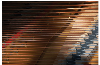
Sit in front of a piano sometime and sing a loud brief note at it with the dampers off its strings (Figure \(\PageIndex{1}\)). It will sing the same note back at you—the strings, having the same frequencies as your voice, are resonating in response to the forces from the sound waves that you sent to them. This is a good example of the fact that objects—in this case, piano strings—can be forced to oscillate, and oscillate most easily at their natural frequency. In this section, we briefly explore applying a periodic driving force acting on a simple harmonic oscillator. The driving force puts energy into the system at a certain frequency, not necessarily the same as the natural frequency of the system. Recall that the natural frequency is the frequency at which a system would oscillate if there were no driving and no damping force.
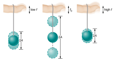
Most of us have played with toys involving an object supported on an elastic band, something like the paddle ball suspended from a finger in Figure \(\PageIndex{2}\). Imagine the finger in the figure is your finger. At first, you hold your finger steady, and the ball bounces up and down with a small amount of damping. If you move your finger up and down slowly, the ball follows along without bouncing much on its own. As you increase the frequency at which you move your finger up and down, the ball responds by oscillating with increasing amplitude. When you drive the ball at its natural frequency, the ball’s oscillations increase in amplitude with each oscillation for as long as you drive it. The phenomenon of driving a system with a frequency equal to its natural frequency is called resonance. A system being driven at its natural frequency is said to resonate. As the driving frequency gets progressively higher than the resonant or natural frequency, the amplitude of the oscillations becomes smaller until the oscillations nearly disappear, and your finger simply moves up and down with little effect on the ball.
Consider a simple experiment. Attach a mass m to a spring in a viscous fluid, similar to the apparatus discussed in the damped harmonic oscillator. This time, instead of fixing the free end of the spring, attach the free end to a disk that is driven by a variable-speed motor. The motor turns with an angular driving frequency of ω . The rotating disk provides energy to the system by the work done by the driving force (Fd = F0 sin(\(\omega\)t)). The experimental apparatus is shown in Figure \(\PageIndex{3}\).
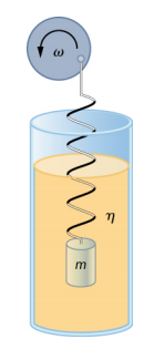
Using Newton’s second law (\(\vec{F}_{net} = m \vec{a}\)), we can analyze the motion of the mass. The resulting equation is similar to the force equation for the damped harmonic oscillator, with the addition of the driving force:
\[-kx -b \frac{dx}{dt} + F_{0} \sin (\omega t) = m \frac{d^{2} x}{dt^{2}} \ldotp \label{15.27}\]
When an oscillator is forced with a periodic driving force, the motion may seem chaotic. The motions of the oscillator is known as transients. After the transients die out, the oscillator reaches a steady state, where the motion is periodic. After some time, the steady state solution to this differential equation is
\[x(t) = A \cos (\omega t + \phi) \ldotp \label{15.28}\]
Once again, it is left as an exercise to prove that this equation is a solution. Taking the first and second time derivative of x(t) and substituting them into the force equation shows that x(t) = Asin(\(\omega t + \phi\)) is a solution as long as the amplitude is equal to
\[A = \frac{F_{0}}{\sqrt{m^{2} (\omega^{2} - \omega_{0}^{2})^{2} + b^{2} \omega^{2}}} \label{15.29}\]
where \(\omega_{0} = \sqrt{\frac{k}{m}}\) is the natural angular frequency of the system of the mass and spring. Recall that the angular frequency, and therefore the frequency, of the motor can be adjusted. Looking at the denominator of the equation for the amplitude, when the driving frequency is much smaller, or much larger, than the natural frequency, the square of the difference of the two angular frequencies \((\omega^{2} − \omega_{0}^{2})^{2}\) is positive and large, making the denominator large, and the result is a small amplitude for the oscillations of the mass. As the frequency of the driving force approaches the natural frequency of the system, the denominator becomes small and the amplitude of the oscillations becomes large. The maximum amplitude results when the frequency of the driving force equals the natural frequency of the system (Amax = \(\frac{F_{0}}{b \omega}\)).
Figure \(\PageIndex{4}\) shows a graph of the amplitude of a damped harmonic oscillator as a function of the frequency of the periodic force driving it. Each of the three curves on the graph represents a different amount of damping. All three curves peak at the point where the frequency of the driving force equals the natural frequency of the harmonic oscillator. The highest peak, or greatest response, is for the least amount of damping, because less energy is removed by the damping force. Note that since the amplitude grows as the damping decreases, taking this to the limit where there is no damping (b = 0), the amplitude becomes infinite.
Note that a small-amplitude driving force can produce a large-amplitude response. This phenomenon is known as resonance. A common example of resonance is a parent pushing a small child on a swing. When the child wants to go higher, the parent does not move back and then, getting a running start, slam into the child, applying a great force in a short interval. Instead, the parent applies small pushes to the child at just the right frequency, and the amplitude of the child’s swings increases.
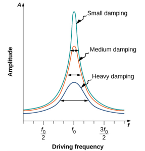
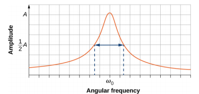
It is interesting to note that the widths of the resonance curves shown in Figure \(\PageIndex{4}\) depend on damping: the less the damping, the narrower the resonance. The consequence is that if you want a driven oscillator to resonate at a very specific frequency, you need as little damping as possible. For instance, a radio has a circuit that is used to choose a particular radio station. In this case, the forced damped oscillator consists of a resistor, capacitor, and inductor, which will be discussed later in this course. The circuit is “tuned” to pick a particular radio station. Here it is desirable to have the resonance curve be very narrow, to pick out the exact frequency of the radio station chosen. The narrowness of the graph, and the ability to pick out a certain frequency, is known as the quality of the system. The quality is defined as the spread of the angular frequency, or equivalently, the spread in the frequency, at half the maximum amplitude, divided by the natural frequency (Q = \(\frac{\Delta \omega}{\omega_{0}}\)) as shown in Figure \(\PageIndex{5}\). For a small damping, the quality is approximately equal to Q ≈ \(\frac{2b}{m}\).
These features of driven harmonic oscillators apply to a huge variety of systems. For instance, magnetic resonance imaging (MRI) is a widely used medical diagnostic tool in which atomic nuclei (mostly hydrogen nuclei or protons) are made to resonate by incoming radio waves (on the order of 100 MHz). In all of these cases, the efficiency of energy transfer from the driving force into the oscillator is best at resonance. Figure \(\PageIndex{6}\) shows the London Millennium Footbridge that allows pedestrians to cross the River Thames in London. This bridge was nicknamed “Wobbly Bridge” when pedestrians experienced swaying motion while crossing it. The bridge was closed for roughly two years to get rid of this motion.

A famous magic trick involves a performer singing a note toward a crystal glass until the glass shatters. Explain why the trick works in terms of resonance and natural frequency.


