6.15: Visualisation and Transformation of Data

This document is a brief overview of a few of the many uses of visualisation and transformation. It also introduces a very useful but little-known technique called a box plot.

You may wish to put the name Edward Tufte into the long term memory store of your brain. He is a true giant in the study of visualisation, and any of his three books on this topic are highly recommended. His most recent one, Visual Explanations : Images and Quantities, Evidence and Narrative includes his work involving the visualisation of verbs! All three books are listed in the References section at the end of this document.

Anscombe's Data

F.W. Anscombe generated a quartet of made-up data in the early 1970's. Each data set has 11 {x,y} pairs of numbers. The means of the x values are almost identical for all four sets; the means of the y values are also almost identical. When we do least-squares fits of the datasets to a straight line we get:

	Intercept	Slope	Sum of the Squares
Set 1	3.00009 ± 0.909545	0.500091 ± 0.0953463	13.7627
Set 2	3.00091 ± 0.909545	0.500000 ± 0.0953463	13.7763
Set 3	3.00245 ± 0.909545	0.499727 ± 0.0953463	13.7562
Set 4	3.00173 ± 0.909545	0.499909 ± 0.0953463	13.7425

So, just looking at the numbers, one might conclude that these four datasets are virtually the same. Note that I have presented the intercepts, slopes and their errors to a ridiculous number of significant figures to illustrate my point.

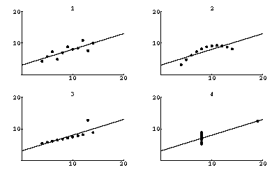When we look at graphs of the data and the fit to them, as to the right, we see that the datasets are quite different.

The fit to dataset 1 is reasonable. The fit to dataset 2 shows that we have used the wrong model; the data does not show a straight line relationship. The fits to datasets 3 and especially 4 illustrate an often ignored problem with least-squares fits: they are not robust and a single datapoint can seize total control of the fit.

This is an illustration of a situation where visualising the data, here by means of a graph, is crucial.

Darwin's Fertilization Data: Introducing the Box Plot

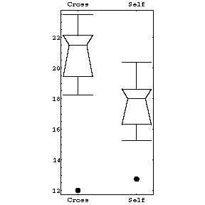
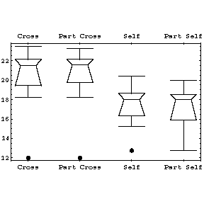
In 1878 Darwin studied the height of 15 mature Zea Mays plants that were cross-fertilised, and compared to the height of 15 plants that were self-fertilised. The results of this early experiment in fertilisation are shown in the histograms to the right.

One concludes that the cross-fertilised plants grew higher than the self-fertilised ones, although one has to study the histograms fairly carefully to reach the conclusion.

To the right we show the same data in a box plot. The plot is explained immediately below.

The "waist" of the box plot is the median. The "shoulder" is the upper quartile, while the "hip" is the lower quartile. Note that these three descriptors are all robust: a single wild data point will have negligible effect. We define H as the height of the "box" (actually trapezoid) and then heuristically define 2 cutoffs as the upper quartile plus 1.5 * H and the lower quartile minus 1.5 * H respectively. The upper "whisker" is the largest data value that is less than the upper cutoff; the lower whisker is the smallest data value that is greater than the lower cutoff. All data points outside the cutoffs are represented as dots; these are called outliers.

Comparing the above histograms and box plots, it is obvious that the box plot shows the differences between the two samples of plants much more clearly.

Darwin threw out the data from pot number 1, which contained three self-fertilised and three cross-fertilised plants. One plant in the pot was diseased, another died, and a third never grew to full height although a reason was never found. The histograms of this data with these plants removed from the sample are shown to the right.
The box plots manage to display so much information at once that we can show all four data sets in a single display. Not only are the differences between cross-fertilised and self-fertilised plants clearly shown, but by using this visualization technique, we see that our conclusion is not effected significantly by throwing out three suspect data points from each sample.

Problem: show that for a Gaussian distribution there is a negligible number of outliers.

Another Box Plot Example

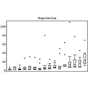To the right we show the population of the 10 largest cities for 16 different countries, as listed in the 1967 World Almanac.

Some of the features that the plots make clear include the fact that for all countries but one (the Netherlands) the largest city is considered an outlier. Also, with only two exceptions, the city populations are skewed towards the larger cities.

The feature of the population data that we will concentrate on is that as the level, the value of the median, increases the spread, the height of the box, also increases. For the more usual case in in Physics of fitting data to curves, the equivalent increase of spread with level would be if the values of the absolute values of the residuals of the fit increased with the value of the independent variable.

One of the problems with data and models in which the level depends on the spread, either increasing or decreasing, is that the common statistical measures called the Analysis of Variance can not be calculated correctly. Thus, more often than is commonly realized, some sort of transformation of the data is required before this system of statistical techniques can be validly used.

For the population data, since populations tend to grow exponentially we are tempted to transform the data by substituting the value of the population for each city with its natural logarithm. The result of doing this transformation is shown to the right. We have largely eliminated the variations in the spread.

By doing this transformation, we have also made the data for the countries with smaller cities much more visible.

Tukey's Ladder of Powers

In the previous section we used some simple insight into population dynamics to guess that a logarithmic transformation might eliminate the dependence of spread on level. Even if we were ignorant of demography, we can show that the data itself suggests a logarithmic transformation.

Suppose that the spread is proportional to a power of the median:

spread = c * medianb

Take the logarithm of both sides:

ln(spread) = ln(c) + b * ln(median)

Thus, if we fit ln(spread) versus ln(median) to a straight line, the slope of the line is b. Then we do a transformation of the data:

trans = original(1 - b)

This will at least approximately eliminate the dependence of spread on level.

In practice, we only estimate (1 - b), which leads to the following table.

b	Transformation
-2	original^3
-1	original^2
0	original (no transformation)
0.5	sqrt(original)
1	ln(original)
1.5	1/sqrt(original)
2	1/original

This is often called Tukey's "ladder of powers".

The transformation ln(original) when b = 1, i.e. (1 - b) is zero, may seem to be artificial, but it is not. In fact x(1-b)behaves much like the logarithm when (1 - b) is close to zero. For example, the derivative of ln(x) is 1/x, and the derivative of x^0.001 is proportional to x^-0.999.

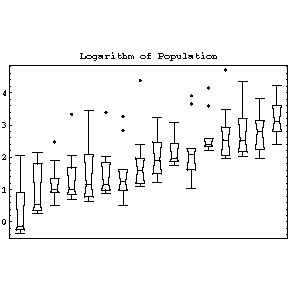
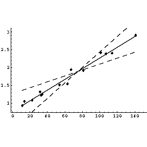
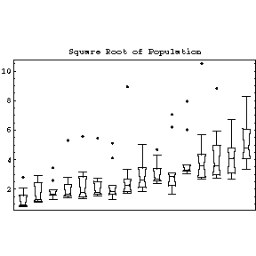If we fit ln(spread) versus ln(level) of the population data to a straight line, the slope of the line turns out to be 0.7 ± 0.3. Thus b is between 0.4 and 1.0. The higher value suggests the logarithmic transformation we examined in the previous section, while the lower value suggests a square-root transformation. The square root transformed data is shown to the right. It too has reduced the dependence of spread on the median, although perhaps not as well as the logarithmic one.

In fact, when in doubt about what transformation to try, the logarithm is a good first guess. The reason is that often the factor we are trying to eliminate is multiplicative instead of additive, such as perhaps some percentage of the variable. A logarithmic transformation will give equal differences in the case of equal multiplicative factors.

An Example of Tukey's Ladder of Powers

We illustrate Tukey's ladder of powers with some data on the growth of the retina of cat fetuses published by Barry Lia, Robert W. Williams, and Leo M Chalupa in Science 236, (1987) pg 848. We fit the data to a parabola and show the graph of the result.
If we plot the absolute value of the residuals versus the independent variable, we see that the magnitude of the residuals is increasing.

If we fit the natural logarithm of the absolute value of the residual versus the logarithm of the value of the independent variable to a straight line, the slope is 0.75 ± 0.44. Thus, from the ladder of powers, either a square root or logarithmic transformation is reasonable. We choose the logarithmic transformation by replacing the value of the dependent variable by its logarithm.

If we fit this transformed data to a straight line, the intercept is 0.774 ± 0.046 and the slope is 0.01499 ± 0.00063. The graph, including the errors in the parameters, is shown to the right.
Examining the absolute value of the residuals, we see that we have essentially eliminated any trends for the value to increase or decrease.

There is some reason to believe that these fits to the transformed data make more sense, both statistically and physically, then fits to the original data.