4.2: Extended Systems and Center of Mass

Consider a collection of particles with masses \(m_1\), \(m_2\),..., and located, at some given instant, at positions \(x_1\), \(x_2\).... (We are still, for the time being, considering only motion in one dimension, but all these results generalize easily to three dimensions.) The center of mass of such a system is a mathematical point whose position coordinate is given by

\[ x_{c m}=\frac{m_{1} x_{1}+m_{2} x_{2}+\ldots}{m_{1}+m_{2}+\ldots} \label{eq:3.8} .\]

Clearly, the denominator of (\ref{eq:3.8}) is just the total mass of the system, which we may just denote by \(M\). If all the particles have the same mass, the center of mass will be somehow “in the middle” of all of them; otherwise, it will tend to be closer to the more massive particle(s). The “particles” in question could be spread apart, or they could literally be the “parts” into which we choose to subdivide, for computational purposes, a single extended object.

If the particles are in motion, the position of the center of mass, \(x_{cm}\), will in general change with time. For a solid object, where all the parts are moving together, the displacement of the center of mass will just be the same as the displacement of any part of the object. In the most general case, we will have (by subtracting \(x_{cmi}\) from \(x_{cmf}\))

\[ \Delta x_{c m}=\frac{1}{M}\left(m_{1} \Delta x_{1}+m_{2} \Delta x_{2}+\ldots\right) \label{eq:3.9} .\]

Dividing Equation (\ref{eq:3.9}) by \(\Delta t\) and taking the limit as \(\Delta t \rightarrow 0\), we get the instantaneous velocity of the center of mass:

\[ v_{c m}=\frac{1}{M}\left(m_{1} v_{1}+m_{2} v_{2}+\ldots\right) \label{eq:3.10} .\]

But this is just

\[ v_{c m}=\frac{p_{s y s}}{M} \label{eq:3.11} .\]

where \(p_{sys} = m_1v_1 + m_2v_2 + \ldots\) is the total momentum of the system.

Center of Mass Motion for an Isolated System

Equation (\ref{eq:3.11}) is a very interesting result. Since the total momentum of an isolated system is constant, it tells us that the center of mass of an isolated system of particles moves at constant velocity, regardless of the relative motion of the particles themselves or their possible interactions with each other. As indicated above, this generalizes straightforwardly to more than one dimension, so we can write \(\vec v_{cm} = \vec p_{sys}/M\). Thus, we can say that, for an isolated system in space, not only the speed, but also the direction of motion of its center of mass does not change with time.

Clearly this result is a sort of generalization of the law of inertia. For a solid, extended object, it does, in fact, provide us with the precise form that the law of inertia must take: in the absence of external forces, the center of mass will just move on a straight line with constant velocity, whereas the object itself may be moving in any way that does not affect the center of mass trajectory. Specifically, the most general motion of an isolated rigid body is a straight line motion of its center of mass at constant speed, combined with a possible rotation of the object as a whole around the center of mass.

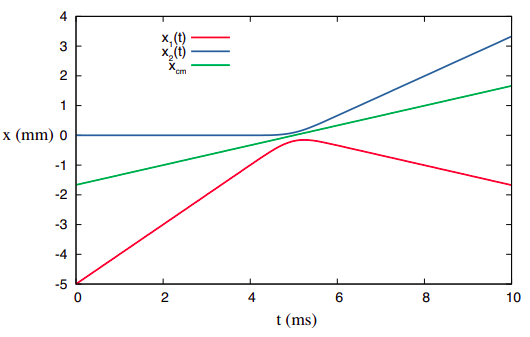
For a system that consists of separate parts, on the other hand, the center of mass is generally just a point in space, which may or may not coincide at any time with the position of any of the parts, but which will nonetheless move at constant velocity as long as the system is isolated. This is illustrated by Figure \(\PageIndex{1}\), where the position vs. time curves have been drawn for the colliding objects of Figure 2.1.1. I have assumed that object 1 starts out at \(x_{1i}\) = −5 mm at \(t\) = 0, and object 2 starts at \(x_{2i}\) = 0 at \(t\) = 0. Because object 2 has twice the inertia of object 1, the position of the center of mass, as given by Equation (\ref{eq:3.8}), will always be

\[ x_{c m}=x_{1} / 3+2 x_{2} / 3 \nonumber \]

that is to say, the center of mass will always be in between objects 1 and 2, and its distance from object 2 will always be half its distance to object 1:

\[ \begin{aligned}
&\left|x_{c m}-x_{1}\right|=\frac{2}{3}\left|x_{1}-x_{2}\right|\\
&\left|x_{c m}-x_{2}\right|=\frac{1}{3}\left|x_{1}-x_{2}\right|
\end{aligned} \]

Figure \(\PageIndex{1}\) shows that this simple prescription does result in motion with constant velocity for the center of mass (the green straight line), even though the \(x\)-vs-\(t\) curves of the two objects themselves look relatively complicated. (Please check it out! Take a ruler to Figure \(\PageIndex{1}\) and verify that the center of mass is, at every instant, where it is supposed to be.)

Figure \(\PageIndex{1}\). The green line shows the position of the center of mass as a function of time.

The concept of center of mass gives us an important way to simplify the description of the motion of potentially complicated systems. We will make good use of it in forthcoming chapters.

A very nice demonstration of the motion of the center of mass in two-body one-dimensional collisions can be found at https://phet.colorado.edu/sims/collision-lab/collision-lab_en.html (you need to check the “center of mass” box to see it).

Defining a System is not Unique

Although we will generally be studying relatively simple systems in the course of this class ("two carts", "a person pulling a sled", etc), it turns out that specifying exactly what things are in the system, and how those things interact, will involve some choices. We hope that these choices do not impact the answers we get, but in some cases they might determine which questions we can actually ask. It will be easiest to illustrate this with a definite example, so we will try to determine the system in the figure shown below, of a tennis racket hitting a ball.

The situation is straightforeward - a person is hitting a ball with a tennis racket. The figure in the center defines this system in what is probably considered the "simplest" fashion, and is generally the approach we will take in this text. The system has two objects ("Ball" and "Racket"). The two objects are interacting with each other, and since both have mass, are also interacting with the Earth via the gravitational force. This will allow us to answer basic questions like "how much force does the ball feel from the racket?" and "how far does the ball travel after it is hit?"

However, consider the figure on the right - it's an alterative, completely correct, definition for this system. In this case, we've broken the racket into three separate objects, "Strings", "Frame", and "Person", each with their own gravitational interactions with the Earth. This is more complicated, but allows us to answer more interesting questions - like "how much force did the frame absorb from the strings?" or, "how much force did the person deliver to the ball?" The original questions are still answerable, but with this more complicated system, we've increased the number of questions we can answer about this seemingly simple system.

As we said, we will generally be focused on the simpler of these systems - the middle one, with a single interaction between the racket and the ball. However, it's worth it to keep in mind that there are tyically a great many other interesting questions that can be answered with the same physical system, it's just a matter of altering the definition of the system. We will sometimes refer to this type of thing as different models for the same physical situation, and we pick which model we want depending on what we want to study about it.