4.3: Reference Frame Changes and Relative Motion

Everything up to this point assumes that we are using a fixed, previously agreed upon reference frame. Basically, this is just an origin and a set of axes along which to measure our coordinates.

There are, however, a number of situations in physics that call for the use of different reference frames, and, more importantly, that require us to convert various physical quantities from one reference frame to another. For instance, imagine you are on a boat on a river, rowing downstream. You are moving with a certain velocity relative to the water around you, but the water itself is flowing with a different velocity relative to the shore, and your actual velocity relative to the shore is the sum of those two quantities. Ships generally have to do this kind of calculation all the time, as do airplanes: the “airspeed” is the speed of a plane relative to the air around it, but that air is usually moving at a substantial speed relative to the earth.

The way we deal with all these situations is by introducing two reference frames, which here I am going to call A and B. One of them, say A, is “at rest” relative to the earth, and the other one is “at rest” relative to something else—which means, really, moving along with that something else. (For instance, a reference frame at rest “relative to the river” would be a frame that’s moving along with the river water, like a piece of driftwood that you could measure your progress relative to.)

In any case, graphically, this will look as in Figure \(\PageIndex{1}\), which we have drawn for the two-dimensional case:

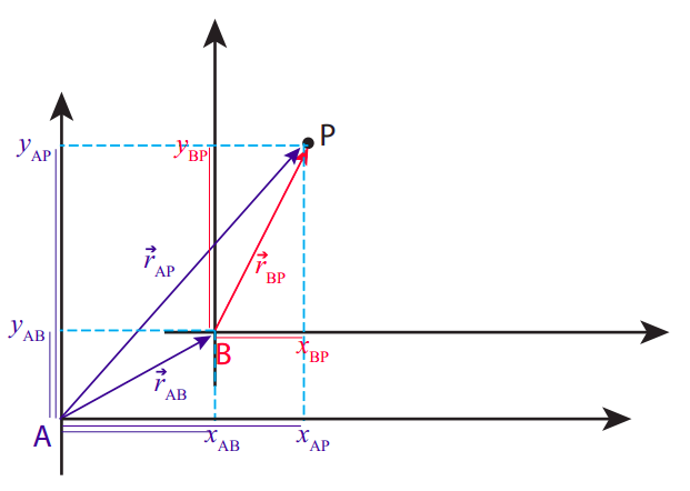
Figure \(\PageIndex{1}\): Position vectors and coordinates of a point P in two different reference frames, A and B.

In the reference frame A, the point P has position coordinates \((x_{AP} , y_{AP})\). Likewise, in the reference frame B, its coordinates are \((x_{BP} , y_{BP})\). As you can see, the notation chosen is such that every coordinate in A will have an “A” as a first subscript, while the second subscript indicates the object to which it refers, and similarly for coordinates in B.

The coordinates \((x_{AB}, y_{AB})\) are special: they are the coordinates, in the reference frame A, of the origin of reference frame B. This is enough to fully locate the frame B in A, as long as the frames are not rotated relative to each other.

The thin colored lines I have drawn along the axes in Figure \(\PageIndex{1}\) are intended to make it clear that the following equations hold:

\[ \begin{array}{l}
{x_{A P}=x_{A B}+x_{B P}} \\
{x_{A P}=x_{A B}+x_{B P}}
\end{array} \label{eq:14} \]

Although the figure is drawn for the easy case where all these quantities are positive, you should be able to convince yourself that Eqs. (\ref{eq:14}) hold also when one or more of the coordinates have negative values.

All these coordinates are also the components of the respective position vectors, shown in the figure and color-coded by reference frame (so, for instance, \(\vec r_{AP}\) is the position vector of P in the frame A), so the equations (\ref{eq:14}) can be written more compactly as the single vector equation

\[ \vec r_{AP} = \vec r_{AB} + \vec r_{BP} \label{eq:15} .\]

From all this you can see how to add vectors: algebraically, you just add their components separately, as in Eqs. (\ref{eq:14}); graphically, you draw them so the tip of one vector coincides with the tail of the other (we call this “tip-to-tail”), and then draw the sum vector from the tail of the first one to the tip of the other one.

Of course, I showed you already how to subtract vectors with Figure 1.2.3: again, algebraically, you just subtract the corresponding coordinates, whereas graphically you draw them with a common origin, and then draw the vector from the tip of the vector you are subtracting to the tip of the other one. If you read the previous paragraph again, you can see that Figure 1.2.3 can equally well be used to show that \(\Delta \vec r = \vec r_f - \vec r_i\), as to show that \(\vec r_f = \vec r_i + \Delta \vec r\).

In a similar way, you can see graphically from Figure \(\PageIndex{1}\) (or algebraically from Equation (\ref{eq:15})) that the position vector of P in the frame B is given by \(\vec r_{BP} = \vec r_{AP} − \vec r_{AB}\). The last term in this expression can be written in a different way, as follows. If I follow the convention I have introduced above, the quantity \(x_{BA}\) (with the order of the subscripts reversed) would be the \(x\) coordinate of the origin of frame A in frame B, and algebraically that would be equal to \(−x_{AB}\), and similarly \(y_{BA} = −y_{AB}\). Hence the vector equality \(\vec r_{AB} = −\vec r_{BA}\) holds. Then,

\[ \vec{r}_{B P}=\vec{r}_{A P}-\vec{r}_{A B}=\vec{r}_{A P}+\vec{r}_{B A} \label{eq:16}. \]

This is, in a way, the “inverse” of Equation (\ref{eq:15}): it tells us how to get the position of P in the frame B if we know its position in the frame A.

Let's show next how all this extends to displacements and velocities. Suppose the point P indicates the position of a particle at the time \(t\). Over a time interval \(\Delta t\), both the position of the particle and the relative position of the two reference frames may change. We can add yet another subscript, \(i\) or \(f\), (for initial and final) to the coordinates, and write, for example,

\[ \begin{array}{l}
{x_{A P, i}=x_{A B, i}+x_{B P, i}} \\
{x_{A P, f}=x_{A B, f}+x_{B P, f}}
\end{array} \label{eq:17} \]

Subtracting these equations gives us the corresponding displacements:

\[ \Delta x_{A P}=\Delta x_{A B}+\Delta x_{B P} \label{eq:18} .\]

Dividing Equation (\ref{eq:18}) by \(\Delta t\) we get the average velocities\(^1\), and then taking the limit \(\Delta t \rightarrow 0\) we get the instantaneous velocities. This applies in the same way to the \(y\) coordinates, and the result is the vector equation

\[ \vec{v}_{A P}=\vec{v}_{B P}+\vec{v}_{A B} \label{eq:19} .\]

We have rearranged the terms on the right-hand side to (hopefully) make it easier to visualize what’s going on. In words: the velocity of the particle P relative to (or measured in) frame A is equal to the (vector) sum of the velocity of the particle as measured in frame B, plus the velocity of frame B relative to frame A.

The result (\ref{eq:19}) is just what we would have expected from the examples mentioned at the beginning of this section, like rowing in a river or an airplane flying in the wind. For instance, for the airplane \(\vec v_{BP}\) could be its “airspeed” (only it has to be a vector, so it would be more like its “airvelocity”: that is, its velocity relative to the air around it), and \(\vec v_{AB}\) would be the velocity of the air relative to the earth (the wind velocity, at the location of the airplane). In other words, A represents the earth frame of reference and B the air, or wind, frame of reference. Then, \(\vec v_{AP}\) would be the “true” velocity of the airplane relative to the earth. You can see how it would be important to add these quantities as vectors, in general, by considering what happens when you fly in a cross wind, or try to row across a river, as in Figure \(\PageIndex{2}\) below.

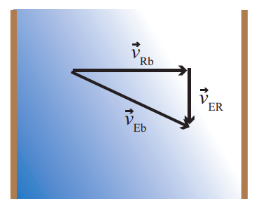
Figure \(\PageIndex{2}\): Rowing across a river. If you head “straight across” the river (with velocity vector \(\vec v_{Rb}\) in the moving frame of the river, which is flowing with velocity \(\vec v_{ER}\) in the frame of the earth), your actual velocity relative to the shore will be the vector \(\vec v_{Eb}\). This is an instance of Equation (\ref{eq:19}), with frame A being E (the earth), frame B being R (the river), and “b” (for “boat”) standing for the point P we are tracking.

As you can see from this couple of examples, Equation (\ref{eq:19}) is often useful as it is written, but sometimes the information we have is given to us in a different way: for instance, we could be given the velocity of the object in frame A \((\vec v_{AP})\), and the velocity of frame B as seen in frame A \((\vec v_{AB})\), and told to calculate the velocity of the object as seen in frame B. This can be easily accomplished if we note that the vector \(\vec v_{AB}\) is equal to \(-\vec v_{BA}\); that is to say, the velocity of frame B as seen from frame A is just the opposite of the velocity of frame A as seen from frame B. Hence, Equation (\ref{eq:19}) can be rewritten as

\[ \vec{v}_{A P}=\vec{v}_{B P}-\vec{v}_{B A} \label{eq:20} .\]

For most of the next few chapters we are going to be considering only motion in one dimension, and so we will write Equation (\ref{eq:19}) (or (\ref{eq:20})) without the vector symbols, and it will be understood that \(v\) refers to the component of the vector \(\vec v\) along the coordinate axis of interest.

A quantity that will be particularly important later on is the relative velocity of two objects, which we could label 1 and 2. The velocity of object 2 relative to object 1 is, by definition, the velocity which an observer moving along with 1 would measure for object 2. So it is just a simple frame change: let the earth frame be frame E and the frame moving with object 1 be frame 1, then the velocity we want is \(v_{12}\) (“velocity of object 2 in frame 1”). If we make the change A \(\rightarrow\) 1, B \(\rightarrow\) E, and P \(\rightarrow\) 2 in Equation (\ref{eq:20}), we get

\[ v_{12}=v_{E 2}-v_{E 1} \label{eq:21} .\]

In other words, the velocity of 2 relative to 1 is just the velocity of 2 minus the velocity of 1. This is again a familiar effect: if you are driving down the highway at 50 miles per hour, and the car in front of you is driving at 55, then its velocity relative to you is 5 mph, which is the rate at which it is moving away from you (in the forward direction, assumed to be the positive one).

It is important to realize that all these velocities are real velocities, each in its own reference frame. Something may be said to be truly moving at some velocity in one reference frame, and just as truly moving with a different velocity in a different reference frame. I will have a lot more to say about this in the next chapter, but in the meantime you can reflect on the fact that, if a car moving at 55 mph collides with another one moving at 50 mph in the same direction, the damage will be basically the same as if the first car had been moving at 5 mph and the second one had been at rest. For practical purposes, where you are concerned, another car’s velocity relative to yours is that car’s “real” velocity.

Resources

A good app for practicing how to add vectors (and how to break them up into components, magnitude and direction, etc.) may be found here:https://phet.colorado.edu/en/simulation/vector-addition.

Perhaps the most dramatic demonstration of how Equation (\ref{eq:19}) works in the real world is in this episode of Mythbusters: https://www.youtube.com/watch?v=BLuI118nhzc. (If this link does not work, do a search for “Mythbusters cancel momentum.”) They shoot a ball from the bed of a truck, with a velocity (relative to the truck) of 60 mph backwards, while the truck is moving forward at 60 mph. I think the result is worth watching.

A very old, but also very good, educational video about different frames of reference is this one: https://www.youtube.com/watch?v=sS17fCom0Ns. You should try to watch at least part of it. Many things will be relevant to later parts of the course, including projectile motion.

---

\(^1\) We have made a very natural assumption, that the time interval \(\Delta t\) is the same for observers tracking the particle’s motion in frames A and B, respectively (where each observer is understood to be moving along with his or her frame). This, however, turns out to be not true when any of the velocities involved is close to the speed of light, and so the simple addition of velocities formula (\ref{eq:19}) does not hold in Einstein’s relativity theory.