8.1: Kinetic Energy

For a long time in the development of classical mechanics, physicists were aware of the existence of two different quantities that one could define for an object of inertia \(m\) and velocity \(v\). One was the momentum, \(mv\), and the other was something proportional to \(mv^2\). Despite their obvious similarities, these two quantities exhibited different properties and seemed to be capturing different aspects of motion.

When things got finally sorted out, in the second half of the 19th century, the quantity \(\frac{1}{2}mv^2\) came to be recognized as a form of energy—itself perhaps the most important concept in all of physics. Kinetic energy, as this quantity is called, may be the most obvious and intuitively understandable kind of energy, and so it is a good place to start our study of the subject.

We will use the letter \(K\) to denote kinetic energy, and, since it is a form of energy, we will express it in the units especially named for this purpose, which is to say joules (J). 1 joule is 1 kg·m²/s². In the definition

\[ K=\frac{1}{2} m v^{2} \label{eq:4.1} \]

the letter \(v\) is meant to represent the magnitude of the velocity vector, that is to say, the speed of the particle. Hence, unlike momentum, kinetic energy is not a vector, but a scalar : there is no sense of direction associated with it. In three dimensions, one could write

\[ K=\frac{1}{2} m\left(v_{x}^{2}+v_{y}^{2}+v_{z}^{2}\right) \label{eq:4.2} \]

There is, therefore, some amount of kinetic energy associated with each component of the velocity vector, but in the end they are all added together in a lump sum.

For a system of particles, we will treat kinetic energy as an additive quantity, just like we did for momentum, so the total kinetic energy of a system will just be the sum of the kinetic energies of all the particles making up the system. Note that, unlike momentum, this is a scalar (not a vector) sum, and most importantly, that kinetic energy is, by definition, always positive, so there can be no question of a “cancellation” of one particle’s kinetic energy by another, again unlike what happened with momentum. Two objects of equal mass moving with equal speeds in opposite directions have a total momentum of zero, but their total kinetic energy is definitely nonzero. Basically, the kinetic energy of a system can never be zero as long as there is any kind of motion going on in the system.

Kinetic Energy in Collisions

To gain some further insights into the concept of kinetic energy, and the ways in which it is different from momentum, it is useful to look at it in the same setting in which we “discovered” momentum, namely, one-dimensional collisions in an isolated system. If we look again at the collision represented in Figure 2.1.1 of Chapter 2, reproduced below,

Figure 8.1.1

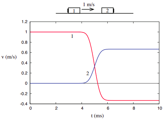
we can use the definition (\ref{eq:4.1}) to calculate the initial and final values of \(K\) for each object, and for the system as a whole. Remember we found that, for this particular system, \(m_2 = 2m_1\), so we can just set \(m_1 \)= 1 kg and \(m_2\) = 2 kg, for simplicity. The initial and final velocities are \(v_{1i}\) = 1 m/s, \(v_{2i}\) = 0, \(v_{1f}\) = −1/3 m/s, \(v_{2f}\) = 2/3 m/s, and so the kinetic energies are

\[ K_{1 i}=\frac{1}{2} \: \mathrm{J}, K_{2 i}=0 ; \quad K_{1 f}=\frac{1}{18} \: \mathrm{J}, K_{2 f}=\frac{4}{9} \: \mathrm{J} \nonumber .\]

Note that 1/18 + 4/9 = 9/18 = 1/2, and so

\[ K_{s y s, i}=K_{1 i}+K_{2 i}=\frac{1}{2} \: \mathrm{J}=K_{1 f}+K_{2 f}=K_{s y s, f} \nonumber .\]

In words, we find that, in this collision, the final value of the total kinetic energy is the same as its initial value, and so it looks like we have “discovered” another conserved quantity (besides momentum) for this system.

This belief may be reinforced if we look next at the collision depicted in Figure 2.1.2, again reproduced below. In this collision, the second object is now moving towards the first, which is stationary.

Figure 8.1.2.

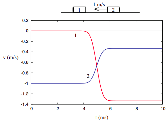
The corresponding kinetic energies are, accordingly, \(K_{1i}\) = 0, \(K_{2i}\) = 1 J, \(K_{1f}\) = \(\frac{8}{9}\) J, \(K_{2f}\) = \(\frac{1}{9}\) J. These are all different from the values we had in the previous example, but note that once again the total kinetic energy after the collision equals the total kinetic energy before—namely, 1 J in this case.

Things are, however, very different when we consider the third collision example shown in Chapter 2, namely, the one where the two objects are stuck together after the collision.

Figure 8.1.3

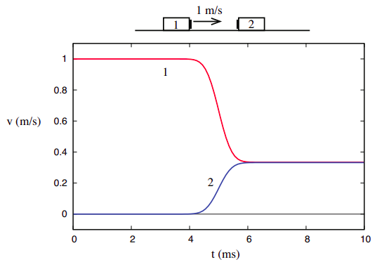
Their joint final velocity, consistent with conservation of momentum, is \(v_{1f}\) = \(v_{2f}\) = 1/3 m/s. Since the system starts as in Figure \(\PageIndex{1}\), its kinetic energy is initially \(K_{sys,i} = \frac{1}{2}\) J, but after the collision we have only

\[ K_{s y s, f}=\frac{1}{2}(3 \: \mathrm{kg})\left(\frac{1}{3} \: \frac{\mathrm{m}}{\mathrm{s}}\right)^{2}=\frac{1}{6} \: \mathrm{J} \nonumber .\]

What this shows, however, is that unlike the total momentum of a system, which is completely unaffected by internal interactions, the total kinetic energy does depend on the details of the interaction, and thus conveys some information about its nature. We can then refine our study of collisions to distinguish two kinds: the ones where the initial kinetic energy is recovered after the collision, which we will call elastic, and the ones where it is not, which we call inelastic. A special case of inelastic collision is the one called totally inelastic, where the two objects end up stuck together, as in Figure \(\PageIndex{3}\). As we shall see later, the kinetic energy “deficit” is largest in that case.

Since whatever ultimately happens depends on the details and the nature of the interaction, we will be led to distinguish between “conservative” interactions, where kinetic energy is reversibly stored as some other form of energy somewhere, and “dissipative” interactions, where the energy conversion is, at least in part, irreversible. Clearly, elastic collisions are associated with conservative interactions and inelastic collisions are associated with dissipative interactions. This preliminary classification of interactions will have to be reviewed a little more carefully, however, in the next chapter.