
9.2: Potential Energy Functions


- Last updated
- Oct 2, 2023
- Save as PDF

( \newcommand{\kernel}{\mathrm{null}\,}\)
It turns out that we can learn quite a lot about some pretty complicated interactions by looking at the functional form of their potential energies. In this section we will look at this, staring with one of the potentials we introducted in the last section, the elastic potential energy.
Imagine that we have two carts collide on an air track, and one of them, let us say cart 2, is fitted with a spring. As the carts come together, they compress the spring, and some of their kinetic energy is “stored” in it as elastic potential energy. In physics, we use the following expression for the potential energy stored in what we call an ideal spring2:
U_s(x)=\frac{1}{2} k\left(x-x_{0}\right)^{2} \label{eq:5.5}
where k is something called the spring constant; x_0 is the “equilibrium length” of the spring (when it is neither compressed nor stretched); and x its actual length, so x>x_0 means the spring is stretched, and x<x_0 means it is compressed. For the system of the two carts colliding, we can take the potential energy to be given by Equation (\ref{eq:5.5}) if the distance between the carts is less than x_0, and 0 (corresponding to a relaxed spring) otherwise. If we put cart 1 on the left and cart 2 on the right, then the distance between them is x_2 − x_1, and so we can write, for the whole interaction
This is enough to solve for the motion of the two carts, given the initial conditions. To see how, look in the “Examples” section at the end of this chapter. Here, I will just give you the result.
For the calculation, shown in Figure \PageIndex{2} below, I have chosen cart 1 to have a mass of 1 kg, an initial position (at t = 0) of x_{1i} = −5 cm and an initial velocity of 1 m/s, whereas cart 2 has a mass of 2 kg and starts at rest at x_{2i} = 0. I have assumed the spring has a length of x_0 = 2 cm and a spring constant k = 1000 J/m2 (which sounds like a lot but isn’t really). The collision begins at t_c = (x_{2i} − x_0 − x_{1i})/v_{1i} = 0.03 s, which is the time it takes cart 1 to travel the 3 cm separating it from the end of the spring. Prior to that point, the total kinetic energy K_{sys} = 0.5 J, and the total potential energy U = 0.
As a result of the collision, the spring compresses and undergoes “half a cycle” of oscillation with an “angular frequency” \omega = \sqrt{k/ \mu} (where \mu is the “reduced mass” of the system, \mu = m_1m_2/(m_1 + m_2)). That is, the spring is compressed and then pushes out until it gets back to its equilibrium length3. This lasts from t = t_c until t = t_c + \pi / \omega, during which time the potential and kinetic energies of the system can be written as
(don’t worry, all this will make a lot more sense after we get to Chapter 11 on simple harmonic motion, I promise!). After t = t_c + \pi / \omega, the interaction is over, and K and U go back to their initial values.
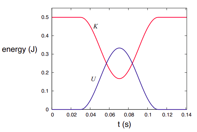
If you compare Figure \PageIndex{2} with Figure 8.2.1 of Chapter 8, you’ll see some similarities. The total energy is always the same, but it might be stored in different forms - motion, springs, or gravity.
2An “ideal spring” is basically defined, mathematically, by this expression, or by the corresponding force equation (which goes by the name of Hooke’s law); usually, we also require that the spring be “massless” (by which we mean that its mass should be negligible compared to all the other masses involved in any given problem). Of course, for Equation (\ref{eq:5.5}) to hold for x < x_0, it must be possible to compress the spring as well as stretch it, which is not always possible with some springs.
3As noted earlier, we shall always assume our springs to be “massless,” that is, that their inertia is negligible. In turn, negligible inertia means that the spring does not “keep going”: it stops stretching as soon as it is back to its original length.
Potential Energy Functions and "Energy Landscapes"
The potential energy function of a system, as illustrated in the above examples, serves to let us know how much energy can be stored in, or extracted from, the system by changing its configuration, that is to say, the positions of its parts relative to each other. We have seen this in the case of the gravitational force (the “configuration” in this case being the distance between the object and the earth), and just now in the case of a spring (how stretched or compressed it is). In all these cases we should think of the potential energy as being a property of the system as a whole, not any individual part; it is, very loosely speaking, something akin to a “stress” in the system that can be turned into motion under the right conditions.
It is a consequence of the principle of conservation of momentum that, if the interaction between two particles can be described by a potential energy function, this should be a function only of their relative position, that is, the quantity x_1 − x_2 (or x_2 − x_1), and not of the individual coordinates, x_1 and x_2, separately4. The example of the spring in the previous section illustrates this, whereas the gravitational potential energy example shows how this can be simplified in an important case: in Equation (9.1.1), the height y of the object above the ground is really a measure of the distance between the object and the earth, something that we could write, in full generality, as |\vec r_o − \vec r_E| (where \vec r_o and \vec r_E are the position vectors of the Earth and the object, respectively). However, since we do not expect the Earth to move very much as a result of the interaction, we can take its position to be constant, and only include the position of the object explicitly in our potential energy function, as we did above5.
Generally speaking, then, we can identify a large class of problems where a “small” object or “particle” interacts with a much more massive one, and it is a good approximation to write the potential energy of the whole system as a function of only the position of the particle. In one dimension, then, we have a situation where, once the initial conditions (the particle’s initial position and velocity) are known, the motion of the particle can be completely determined from the function U(x), where x is the particle’s position at any given time. This can be done using calculus (namely, let v=\pm \sqrt{2 m(E-U(x))} and solve the resulting differential equation); but it is also possible to get some pretty valuable insights into the particle’s motion without using any calculus at all, through a mostly graphical approach that I would like to show you next.
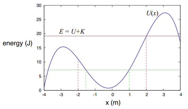
In Figure \PageIndex{3} above I have assumed, as an example, that the potential energy of the system, as a function of the position of the particle, is given by the function U(x) = −x^4/4+9x^2/2+2x + 1 (in joules, if x is given in meters). Consider then what happens if the particle has a mass m = 4 kg and is found initially at x_i = −2 m, with a velocity v_i = 2 m/s. (This scenario goes with the red lines in Figure \PageIndex{3}, so please ignore the green lines for the time being.) Its kinetic energy will then be K_i = 8 J, whereas the potential energy will be U(−2) = 11 J. The total mechanical energy is then E = 19 J, as indicated by the red horizontal line.
Now, as the particle moves, the total energy remains constant, so as it moves to the right, its potential energy goes down at first, and consequently its kinetic energy goes up—that is, it accelerates. At some point, however (around x = −0.22 m) the potential energy starts to go up, and so the particle starts to slow down, although it keeps going, because K = E − U is still nonzero. However, when the particle eventually reaches the point x = 2 m, the potential energy U(2) = 19 J, and the kinetic energy becomes zero.
At that point, the particle stops and turns around, just like an object thrown vertically upwards. As it moves “down the potential energy hill,” it recovers the kinetic energy it used to have, so that when it again reaches the starting point x = −2 m, its speed is again 2 m/s, but now it is moving in the opposite direction, so it just passes through and over the next “hill” (since it has enough total energy to do so), and eventually moves outside the region shown in the figure.
As another example, consider what would have happened if the particle had been released at, say, x = 1 m, but with zero velocity. (This is illustrated by the green lines in Figure \PageIndex{3}.) Then the total energy would be just the potential energy U(1) = 7.25 J. The particle could not possibly move to the right, since that would require the total energy to go up. It can only move to the left, since in that direction U(x) decreases (initially, at first), and that means K can increase (recall K is always positive as long as the particle is in motion). So the particle speeds up to the left until, past the point x = −0.22 m, U(x) starts to increase again and K has to go down. Eventually, as the figure shows, we reach a point (which we can calculate to be x = −1.548 m) where U(x) is once again equal to 7.25 J. This leaves no room for any kinetic energy, so the particle has to stop and turn back. The resulting motion consists of the particle oscillating back and forth forever between x = −1.548 m and x = 1 m.
At this point, you may have noticed that the motion I have described as following from the U(x) function in Figure \PageIndex{3} resembles very much the motion of a car on a roller-coaster having the shape shown, or maybe a ball rolling up and down hills like the ones shown in the picture. In fact, the correspondence can be made exact—if we substitute sliding for rolling, since rolling motion has complications of its own. Given an arbitrary potential energy function U(x) for a particle of mass m, imagine that you build a “landscape” of hills and valleys whose height y above the horizontal, for a given value of the horizontal coordinate x, is given by the function y(x) = U(x)/mg. (Note that mg is just a constant scaling factor that does not change the shape of the curve.) Then, for an object of mass m sliding without friction over that landscape, under the influence of gravity, the gravitational potential energy at any point x would be U^G(x) = mgy = U(x), and therefore its speed at any point will be precisely the same as that of the original particle, if it starts at the same point with the same velocity
This notion of an “energy landscape” can be extended to more than one dimension (although they are hard to visualize in three!), or generalized to deal with configuration parameters other than a single particle’s position. It can be very useful in a number of disciplines (not just physics), to predict the ways in which the configuration of a system may be likely to change.
4We will see why in the next chapter!
5This will change in Chapter 13, when we get to study gravity over a planetary scale.