
13.4: Examples
- Page ID
- 63196

\( \newcommand{\vecs}[1]{\overset { \scriptstyle \rightharpoonup} {\mathbf{#1}} } \)
\( \newcommand{\vecd}[1]{\overset{-\!-\!\rightharpoonup}{\vphantom{a}\smash {#1}}} \)
\( \newcommand{\dsum}{\displaystyle\sum\limits} \)
\( \newcommand{\dint}{\displaystyle\int\limits} \)
\( \newcommand{\dlim}{\displaystyle\lim\limits} \)
\( \newcommand{\id}{\mathrm{id}}\) \( \newcommand{\Span}{\mathrm{span}}\)
( \newcommand{\kernel}{\mathrm{null}\,}\) \( \newcommand{\range}{\mathrm{range}\,}\)
\( \newcommand{\RealPart}{\mathrm{Re}}\) \( \newcommand{\ImaginaryPart}{\mathrm{Im}}\)
\( \newcommand{\Argument}{\mathrm{Arg}}\) \( \newcommand{\norm}[1]{\| #1 \|}\)
\( \newcommand{\inner}[2]{\langle #1, #2 \rangle}\)
\( \newcommand{\Span}{\mathrm{span}}\)
\( \newcommand{\id}{\mathrm{id}}\)
\( \newcommand{\Span}{\mathrm{span}}\)
\( \newcommand{\kernel}{\mathrm{null}\,}\)
\( \newcommand{\range}{\mathrm{range}\,}\)
\( \newcommand{\RealPart}{\mathrm{Re}}\)
\( \newcommand{\ImaginaryPart}{\mathrm{Im}}\)
\( \newcommand{\Argument}{\mathrm{Arg}}\)
\( \newcommand{\norm}[1]{\| #1 \|}\)
\( \newcommand{\inner}[2]{\langle #1, #2 \rangle}\)
\( \newcommand{\Span}{\mathrm{span}}\) \( \newcommand{\AA}{\unicode[.8,0]{x212B}}\)
\( \newcommand{\vectorA}[1]{\vec{#1}} % arrow\)
\( \newcommand{\vectorAt}[1]{\vec{\text{#1}}} % arrow\)
\( \newcommand{\vectorB}[1]{\overset { \scriptstyle \rightharpoonup} {\mathbf{#1}} } \)
\( \newcommand{\vectorC}[1]{\textbf{#1}} \)
\( \newcommand{\vectorD}[1]{\overrightarrow{#1}} \)
\( \newcommand{\vectorDt}[1]{\overrightarrow{\text{#1}}} \)
\( \newcommand{\vectE}[1]{\overset{-\!-\!\rightharpoonup}{\vphantom{a}\smash{\mathbf {#1}}}} \)
\( \newcommand{\vecs}[1]{\overset { \scriptstyle \rightharpoonup} {\mathbf{#1}} } \)
\(\newcommand{\longvect}{\overrightarrow}\)
\( \newcommand{\vecd}[1]{\overset{-\!-\!\rightharpoonup}{\vphantom{a}\smash {#1}}} \)
\(\newcommand{\avec}{\mathbf a}\) \(\newcommand{\bvec}{\mathbf b}\) \(\newcommand{\cvec}{\mathbf c}\) \(\newcommand{\dvec}{\mathbf d}\) \(\newcommand{\dtil}{\widetilde{\mathbf d}}\) \(\newcommand{\evec}{\mathbf e}\) \(\newcommand{\fvec}{\mathbf f}\) \(\newcommand{\nvec}{\mathbf n}\) \(\newcommand{\pvec}{\mathbf p}\) \(\newcommand{\qvec}{\mathbf q}\) \(\newcommand{\svec}{\mathbf s}\) \(\newcommand{\tvec}{\mathbf t}\) \(\newcommand{\uvec}{\mathbf u}\) \(\newcommand{\vvec}{\mathbf v}\) \(\newcommand{\wvec}{\mathbf w}\) \(\newcommand{\xvec}{\mathbf x}\) \(\newcommand{\yvec}{\mathbf y}\) \(\newcommand{\zvec}{\mathbf z}\) \(\newcommand{\rvec}{\mathbf r}\) \(\newcommand{\mvec}{\mathbf m}\) \(\newcommand{\zerovec}{\mathbf 0}\) \(\newcommand{\onevec}{\mathbf 1}\) \(\newcommand{\real}{\mathbb R}\) \(\newcommand{\twovec}[2]{\left[\begin{array}{r}#1 \\ #2 \end{array}\right]}\) \(\newcommand{\ctwovec}[2]{\left[\begin{array}{c}#1 \\ #2 \end{array}\right]}\) \(\newcommand{\threevec}[3]{\left[\begin{array}{r}#1 \\ #2 \\ #3 \end{array}\right]}\) \(\newcommand{\cthreevec}[3]{\left[\begin{array}{c}#1 \\ #2 \\ #3 \end{array}\right]}\) \(\newcommand{\fourvec}[4]{\left[\begin{array}{r}#1 \\ #2 \\ #3 \\ #4 \end{array}\right]}\) \(\newcommand{\cfourvec}[4]{\left[\begin{array}{c}#1 \\ #2 \\ #3 \\ #4 \end{array}\right]}\) \(\newcommand{\fivevec}[5]{\left[\begin{array}{r}#1 \\ #2 \\ #3 \\ #4 \\ #5 \\ \end{array}\right]}\) \(\newcommand{\cfivevec}[5]{\left[\begin{array}{c}#1 \\ #2 \\ #3 \\ #4 \\ #5 \\ \end{array}\right]}\) \(\newcommand{\mattwo}[4]{\left[\begin{array}{rr}#1 \amp #2 \\ #3 \amp #4 \\ \end{array}\right]}\) \(\newcommand{\laspan}[1]{\text{Span}\{#1\}}\) \(\newcommand{\bcal}{\cal B}\) \(\newcommand{\ccal}{\cal C}\) \(\newcommand{\scal}{\cal S}\) \(\newcommand{\wcal}{\cal W}\) \(\newcommand{\ecal}{\cal E}\) \(\newcommand{\coords}[2]{\left\{#1\right\}_{#2}}\) \(\newcommand{\gray}[1]{\color{gray}{#1}}\) \(\newcommand{\lgray}[1]{\color{lightgray}{#1}}\) \(\newcommand{\rank}{\operatorname{rank}}\) \(\newcommand{\row}{\text{Row}}\) \(\newcommand{\col}{\text{Col}}\) \(\renewcommand{\row}{\text{Row}}\) \(\newcommand{\nul}{\text{Nul}}\) \(\newcommand{\var}{\text{Var}}\) \(\newcommand{\corr}{\text{corr}}\) \(\newcommand{\len}[1]{\left|#1\right|}\) \(\newcommand{\bbar}{\overline{\bvec}}\) \(\newcommand{\bhat}{\widehat{\bvec}}\) \(\newcommand{\bperp}{\bvec^\perp}\) \(\newcommand{\xhat}{\widehat{\xvec}}\) \(\newcommand{\vhat}{\widehat{\vvec}}\) \(\newcommand{\uhat}{\widehat{\uvec}}\) \(\newcommand{\what}{\widehat{\wvec}}\) \(\newcommand{\Sighat}{\widehat{\Sigma}}\) \(\newcommand{\lt}{<}\) \(\newcommand{\gt}{>}\) \(\newcommand{\amp}{&}\) \(\definecolor{fillinmathshade}{gray}{0.9}\)In the early days of space flight, astronauts sometimes mentioned the counterintuitive aspects of orbital flight. For example, if, from a circular orbit around the Earth, they wanted to move to a lower orbit, the way to do it was to slow down their capsule (by firing a thruster in the direction opposite their motion). This would take them to a lower orbit, but then the capsule would start speeding up, on its own.
Use the concepts introduced in this chapter to explain what is going on in this scenario. Let \(R\) be the radius of the initial orbit. For simplicity, assume the thruster is on only for a very short time, so you can neglect the motion of the capsule during this time. In other words, treat it as an instantaneous reduction in velocity, and discuss:
- What happens to the system’s potential and kinetic energy, and angular momentum?
- Is the new orbit circular or elliptic? How do you know? What is the new orbit’s \(r_{max}\) (maximum distance to the center of the Earth)?
- Why does the capsule speed up in its new orbit?
- If the new orbit is not circular, what would the astronauts need to do to make it so? (Without getting any closer to the Earth, that is, keeping \(r_{min}\) the same.)
Make sure to draw a diagram of the situation. Make it as accurate as you can.
Solution
(a) Under the assumption that the capsule barely changes position during the thruster firing, the potential energy of the system, which is equal to \(U^G = −GMm/R\), will not change: \(U^G_f = U^G_i\).
The kinetic energy, on the other hand, will go down, since the capsule’s speed is reduced: \(K_f < K_i\). Hence, the total mechanical energy of the system, \(E = K + U^G\), will decrease: \(E_f < E_i\).
The angular momentum will go down, since v goes down.
(b) The new orbit has to be elliptical, since to have a circular orbit at a distance \(R\) requires a precise velocity (given just below Equation (10.1.11) by \(v=\sqrt{G M / R}\)), and now we have changed that.
However, since the orbit must still be a closed curve, it will contain the starting point, which is, by our assumption, a distance \(R\) away from the Earth. Also, if the direction of the velocity vector does not change as a result of the thruster firing (only the magnitude of \(v\) is supposed to change), it follows that at this point the velocity and the position vectors are perpendicular. For a circular orbit, this is the case everywhere. For an elliptical orbit, this is only true at the two extreme points labeled P and A in Figure 10.1.3 (the perigee and apogee, respectively). So, the initial position of the capsule becomes either the perigee or the apogee of the new orbit. Which is it?
To get the answer, recall that we found in (a) that the total mechanical energy \(E\) has gone down. But, since \(E\) is a negative number, this means the magnitude of \(E\) has gone up. Then, in the formula (10.1.14),
\[ E=-\frac{G M m}{2 a} \nonumber \]
the semimajor axis \(a\) must have gone down. For the original circular orbit, we had \(a = R\); now, we must have \(a < R\). This means that the starting point, a distance \(R\) away from the (center of the) Earth, cannot be the perigee (the point of closest approach), since at that point \(r = r_{min}\), and \(r_{min}\) is always less than \(a\) (check again Figure 10.1.3, or Eqs. (10.1.12)). Instead, the starting point has to be the apogee of the new orbit, and therefore the distance at that point is also the maximum distance: \(r_{max} = R\).
(c) The capsule speeds up in its new orbit because, as we just saw, it starts as far away from the Earth as it’s going to get; therefore, as it moves it will start getting closer to the Earth, and we know from Kepler’s second law that as it gets closer it has to speed up. (You can also say that, as it gets closer, the gravitational potential energy of the system will go down, and therefore its kinetic energy must increase.)
(d) The easiest way to change the new orbit to a circular orbit with radius \(r_{min}\) would be to perform another speed-reduction maneuver, but this time at perigee. At perigee, the distance to the Earth is already \(r_{min}\), which is what you want it to be, but the capsule is moving too fast to stay on a circular orbit (put differently, the gravitational force of the Earth at that point is too weak to bend the orbit into a circle): that is why it eventually ends up “overshooting” the Earth on the other side. Reducing \(v\) will further reduce \(E\) and, by the same argument as above, it will result in an orbit with a smaller \(a\), which is what you want (since, at the moment, \(a > r_{min}\), and you want the new \(a\) to be equal to \(r_{min}\)).
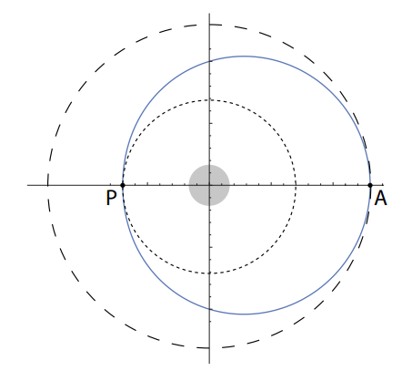
The diagram of the situation is above (previous page). The long-dash circle is the original orbit; the solid line is the elliptical orbit resulting from the speed reduction at point A; the short-dash circle is the circular orbit that would result from another speed reduction at the point P. Note: the size of the orbits is greatly exaggerated compared to those in the early space flights, which were much closer to the Earth!
The way to draw this kind of figure is to first draw an accurate ellipse, making sure you know where the focus is; then draw the circles centered at the focus and touching the ellipse at the right points. An ellipse’s equation in polar form, with the origin at one focus, is \(r = a + ae \cos \phi\).
Example \(\PageIndex{2}\): orbital data from observations- halley's comet
Halley’s comet follows an elliptical orbit around the sun. At its closest approach, it is a distance of 0.59 AU from the sun (an astronomical unit, AU, is defined as the average distance from the earth to the sun: 1 AU = 1.496 × 10¹¹ m), and it is moving at 5.4 × 10⁴ m/s. We know its period is approximately 76 years. Ignoring the forces exerted on the comet by the other solar system objects (a rather rough approximation):
- Use the appropriate Kepler law to infer the value of a (the semimajor axis) for the comet’s orbit.
- What is the eccentricity of the comet's orbit?
- Using the result in (a) and conservation of angular momentum, find the speed of the comet at aphelion (the point in its orbit when it is farthest away from the sun).
Solution
(a) The “appropriate Kepler law” here is the third one. For any two objects orbiting, for instance, the sun, the square of their orbital periods is proportional to the cube of their orbits’ semimajor axes, with the same proportionality constant (\(4\pi/GM_{sun}\); see Equation (10.1.18)). We do not even need to calculate the proportionality constant; we can divide the equation for Halley’s comet by the equation for the earth, and get
\[ \frac{T_{\text {Halley }}^{2}}{T_{\text {earth }}^{2}}=\frac{a_{\text {Halley }}^{3}}{a_{\text {earth }}^{3}} \label{eq:10.21} \]
where \(T^2_{earth}\) = 1 yr2, and \(a^3_{earth}\) = 1 AU3, so we get immediately
\[ a_{\text {Halley }}=\left(76^{2}\right)^{1 / 3} \mathrm{AU}=17.9 \: \mathrm{AU} \label{eq:10.22} \]
(b) We can get this one from a look at Figure 10.1.3: the product \(ea\), plus the minimum distance between the comet and the sun (0.59 AU) is equal to \(a\). (This is just what the second of the equations (10.1.12) says as well.). So we have
\[ e=\frac{a-r_{\min }}{a}=1-\frac{r_{\min }}{a}=1-\frac{0.59}{17.9}=0.967 \label{eq:10.23} \]
Note that we did not even have to convert AU to kilometers. In these types of problems, particularly, where you have to manipulate very large numbers, it really pays off to do all the calculations symbolically and not substitute the numbers in until the very end, to see if something cancels out, and to prevent mistakes when copying large numbers form one line to the next; and sometimes, like here, you do not even have to convert to other units!
(c) At the point of closest approach (perihelion), the velocity and the position vector of the comet are perpendicular, and so the magnitude of the comet’s angular momentum is just equal to \(L = mrv\). The same happens at the farthest point in the orbit (aphelion), and since angular momentum is conserved for the Kepler problem, we can write
\[ m r_{\min } v_{\max }=m r_{\max } v_{\min } \label{eq:10.24} \]
(the reason for this choice of subscripts is that we know that when \(r\) is maximum, \(v\) is minimum, and vice-versa). Solving for \(v_{min}\), the speed at aphelion, we get
\[ v_{\min }=\frac{r_{\min }}{r_{\max }} v_{\max }=\frac{r_{\min }}{2 a-r_{\min }} v_{\max }=\frac{0.59}{2 \cdot 17.9-0.59} 5.4 \times 10^{4} \: \frac{\mathrm{m}}{\mathrm{s}}=905 \: \frac{\mathrm{m}}{\mathrm{s}} \label{eq:10.25} .\]
Here again the equation I used to find \(r_{max}\) can be derived directly from Figure 10.1.3 (and it is also one of the equations (10.1.12): \(r_{min} + r_{max} = 2a\)). Once again, I was able to use AU throughout, since the units of distance cancel out in the fraction \(r_{min}/r_{max}\).