16.1: Dealing with Forces in Two Dimensions

We have been able to get a lot of physics from our study of (mostly) one-dimensional motion only, but it goes without saying that the real world is a lot richer than that, and there are a number of new and interesting phenomena that appear when one considers motion in two or three dimensions. The purpose of this chapter is to introduce you to some of the simplest two-dimensional situations of physical interest.

A common feature to all these problems is that the forces acting on the objects under consideration will typically not line up with the displacements. This means, in practice, that we need to pay more attention to the vector nature of these quantities than we have done so far. This section will present a brief reminder of some basic properties of vectors, and introduce a couple of simple principles for the analysis of the systems that will follow.

To begin with, recall that a vector is a quantity that has both a magnitude and a direction. The magnitude of the vector just tells us how big it is: the magnitude of the velocity vector, for instance, is the speed, that is, just how fast something is moving. When working with vectors in one dimension, we have typically assumed that the entire vector (whether it was a velocity, an acceleration or a force) lay along the line of motion of the system, and all we had to do to indicate the direction was to give the vector’s magnitude an appropriate sign. For the problems that follow, however, it will become essential to break up the vectors into their components along an appropriate set of axes. This involves very simple geometry, and follows the example of the position vector \(\vec r\), whose components are just the Cartesian coordinates of the point it locates in space (as shown in Figure \(\PageIndex{1}\)). For a generic vector, for instance, a force, like the one shown in Figure \(\PageIndex{1}\) below, the components \(F_x\) and \(F_y\) may be obtained from a right triangle, as indicated there:

Figure \(\PageIndex{1}\): : The components of a vector that makes an angle \(\theta\) with the positive \(x\) axis. Two examples are shown, for \(\theta < 90^{\circ}\) (in which case \(F_x \)> 0) and for \(90^{\circ} < \theta < 180^{\circ}\) (in which case \(F_x\) < 0). In both cases, \(F_y\) > 0.

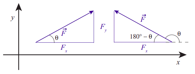
The triangle will always have the vector’s magnitude (\(|\vec{F}|\) in this case) as the hypothenuse. The two other sides should be parallel to the coordinate axes. Their lengths are the corresponding components, except for a sign that depends on the orientation of the vector. If we happen to know the angle \(\theta\) that the vector makes with the positive \(x\) axis, the following relations will always hold:

\begin{align}
F_{x} &=|\vec{F}| \cos \theta \nonumber \\
F_{y} &=|\vec{F}| \sin \theta \nonumber \\
|\vec{F}| &=\sqrt{F_{x}^{2}+F_{y}^{2}} \nonumber \\
\theta &=\tan ^{-1} \frac{F_{y}}{F_{x}} \label{eq:8.1}.
\end{align}

Note, however, that in general this angle \(\theta\) may not be one of the interior angles of the triangle (as shown on the right diagram in Figure \(\PageIndex{1}\)), and that in that case it may just be simpler to calculate the magnitude of the components using trigonometry and an interior angle (such as 180\(^{\circ} − \theta\) in the example), and give them the appropriate signs “by hand.” In the example on the right, the length of the horizontal side of the triangle is equal to \( |\vec{F}| \cos \left(180^{\circ}-\theta\right) \), which is a positive quantity; the correct value for \(F_x\), however, is the negative number \(|\vec{F}| \cos \theta=-|\vec{F}| \cos \left(180^{\circ}-\theta\right)\).

In any case, it is important not to get fixated on the notion that “the \(x\) component will always be proportional to the cosine of \(\theta\).” The symbol \(\theta\) is just a convenient one to use for a generic angle. There are four sections in this chapter, and in every one there is a \(\theta\) used with a different meaning. When in doubt, just draw the appropriate right triangle and remember from your trigonometry classes which side goes with the sine, and which with the cosine (remember SOHCAHTOA!).

For the problems that we are going to study in this chapter, the idea is to break up all the forces involved into components along properly-chosen coordinate axes, then add all the components along any given direction, and apply \(F_{net} = ma\) along that direction: that is to say, we will write (and eventually solve) the equations

\begin{align}
&F_{n e t, x}=m a_{x} \nonumber \\
&F_{n e t, y}=m a_{y} \label{eq:8.2}.
\end{align}

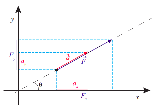
We can show that Eqs. (\ref{eq:8.2}) must hold for any choice of orthogonal \(x\) and \(y\) axes, based on the fact that we know \(\vec F_{net} = m\vec a\) holds along one particular direction, namely, the direction common to \(\vec F_{net}\) and \(\vec a\), and the fact that we have defined the projection procedure to be the same for any kind of vector. Figure \(\PageIndex{2}\) shows how this works. Along the dashed line you just have the situation that is by now familiar to us from one-dimensional problems, where \(\vec a\) lies along \(\vec F\) (assumed here to be the net force), and \( |\vec{F}|=m|\vec{a}|\). However, in the figure I have chosen the axes to make an angle \(\theta\) with this direction. Then, if you look at the projections of \(\vec F\) and \(\vec a\) along the \(x\) axis, you will find

\begin{align}
a_{x}&=|\vec{a}| \cos \theta \nonumber \\
F_{x}&=|\vec{F}| \cos \theta=m|\vec{a}| \cos \theta=m a_{x} \label{eq:8.3}
\end{align}

and similarly, \(F_y = ma_y\). In words, each component of the force vector is responsible for only the corresponding component of the acceleration. A force in the \(x\) direction does not cause any acceleration in the \(y\) direction, and vice-versa.

Figure \(\PageIndex{2}\): If you take the familiar, one-dimensional (see the black dashed line) form of \(\vec F = m\vec a\), and project it onto orthogonal, rotated axes, you get the general two-dimensional case, showing that each orthogonal component of the acceleration is proportional, via the mass \(m\), to only the corresponding component of the force (Eqs. (\ref{eq:8.2})).

In the rest of the chapter we shall see how to use Eqs. (\ref{eq:8.2}) in a number of examples. One thing I can anticipate is that, in general, we will try to choose our axes (unlike in Figure \(\PageIndex{2}\) above) so that one of them does coincide with the direction of the acceleration, so the motion along the other direction is either nonexistent (\(v\) = 0) or trivial (constant velocity).