16.2: Motion in Two Dimensions and Projectile Motion
- Page ID
- 63331
Motion in Two Dimensions and Projectile Motion
So far, we have studied motion under constant acceleration in one-dimension only. In this case, an object is restricted to move in a line (i.e. only along the x or y-directions), and the kinematic equations describe how the object moves. In this section, we will start looking at objects moving in two dimensions. A primary application of this topic is the study of objects moving in the gravitational field, which is called projectile motion.
Motion in Two Dimensions
How do we know when an object is moving in one dimension or two dimensions? The first answer to this is that it might depend on the coordinate system we choose. For instance, consider a car traveling at a constant speed in the north-west direction. In the coordinate system with x along east and y along north, the car is moving in two dimensions. However, if we pick a coordinate system which is tilted 45\( ^\circ \) with respect to the earth-north one, we can describe this car as only moving in one dimension.
However, we don't always have this choice. A better answer is to consider the vectors which describe the object's motion, \(\vec{r}(t)\), \(\vec{v}(t)\), and \(\vec{a}(t)\). If an object has either velocity or acceleration in more then one direction, then the object will move in more than one direction. Notice we have to consider both velocity and acceleration. For example, if we have an object with initial velocity in the x-direction, but acceleration in the y:
\[\vec{v}(t)=v_0\hat{x},\qquad \vec{a}(t)=a_y\hat{y},\]
then although the motion is initially just along the x-axis, the object will start to accelerate along the y-axis almost immediately. At some point later, the velocity will be
\[\vec{v}(t)=v_0\hat{x}+v_y(t)\hat{y},\]
where \(v_y(t)\) is the velocity after undergoing the acceleration \(a_y\) for some time interval.
Constant Acceleration in Two Directions
If you recall, in order to derive the kinematic equations in one-dimension, we started with the basic definition
\[a_x=\frac{dv_x}{dt},\]
and integrated twice with respect to time (review those equations now if you don't remember them!). That required us to add in the initial values \(x_0\) for the position and \(v_{0x}\) for the velocity. We didn't include anything about the y-direction because we assumed the acceleration in the y-direction was zero. But if that's not true, we would simply have
\[a_y=\frac{dv_y}{dt},\]
and we could repeat the same analysis that we performed in the y-direction. In the end, we would end up with two copies of the kinematic equations, one in the x-direction and one in the y-direction,
\[x(t)=\frac{1}{2}a_xt^2+v_{0x}t+x_0,\quad v_x(t)=a_xt+v_{0x},\quad y(t)=\frac{1}{2}a_yt^2+v_{0y}t+y_0,\quad v_y(t)=a_yt+v_{0y}\]
A key feature here is that the two directions are connected by the time and nothing else. Each direction has its own set of initial and final position, velocity, and acceleration, but they are parametrized by time. This means that finding the time interval under consideration is often the best way to solve any particular problem.
Projectile Motion
A particular case of two-dimensional motion under constant acceleration is projectile motion. In this case, we want to study the motion of an object which has only a single force acting on it, that of gravity. Often, this is an object which we throw, or propel into the air in some way. Since we usually don't know anything how how it is thrown (by hand? by canon? by gun?), we start our analysis right after it is in motion, when only gravity is acting on it.
If gravity is the only force acting on the object, we can say right away what the magnitude of the acceleration is, \(a=g=9.81\) m/s\(^2\). It is also most convienient to set the coordinate system so that the y-direction is downwards, so that
\[\vec{a}=-g\hat{y}.\]
In other words, the acceleration in the x-direction is zero, \(a_x=0\). This will greatly simplify the kinematic equations, but we have to be a little careful - just because there is no acceleration in the x-direction does not mean there is no motion in the x-direction. If you throw an object into the air at an arbitrary angle, it will move in both the x- and y-directions, even though it will only accelerate downwards.
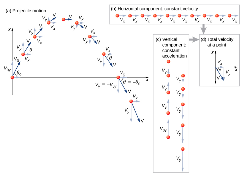
- Resolve the motion into horizontal and vertical components along the x- and y-axes. The magnitudes of the components of displacement \(\vec{s}\) along these axes are x and y. The magnitudes of the components of velocity \(\vec{v}\) are vx = vcos\(\theta\) and vy = vsin\(\theta\), where v is the magnitude of the velocity and \(\theta\) is its direction relative to the horizontal, as shown in Figure \(\PageIndex{2}\).
- Treat the motion as two independent one-dimensional motions: one horizontal and the other vertical. Use the kinematic equations for horizontal and vertical motion presented earlier.
- Solve for the unknowns in the two separate motions: one horizontal and one vertical. Note that the only common variable between the motions is time t. The problem-solving procedures here are the same as those for one-dimensional kinematics and are illustrated in the following solved examples.
- Recombine quantities in the horizontal and vertical directions to find the total displacement \(\vec{s}\) and velocity \(\vec{v}\). Solve for the magnitude and direction of the displacement and velocity using \(s = \sqrt{x^{2} + y^{2}} \ldotp \quad \phi = \tan^{-1} \left(\dfrac{y}{x}\right), \quad v = \sqrt{v_{x}^{2} + v_{y}^{2}} \ldotp\)where \(\phi\) is the direction of the displacement \(\vec{s}\).