
21.2: Work Done on a System By All the External Forces
- Page ID
- 63184

\( \newcommand{\vecs}[1]{\overset { \scriptstyle \rightharpoonup} {\mathbf{#1}} } \)
\( \newcommand{\vecd}[1]{\overset{-\!-\!\rightharpoonup}{\vphantom{a}\smash {#1}}} \)
\( \newcommand{\id}{\mathrm{id}}\) \( \newcommand{\Span}{\mathrm{span}}\)
( \newcommand{\kernel}{\mathrm{null}\,}\) \( \newcommand{\range}{\mathrm{range}\,}\)
\( \newcommand{\RealPart}{\mathrm{Re}}\) \( \newcommand{\ImaginaryPart}{\mathrm{Im}}\)
\( \newcommand{\Argument}{\mathrm{Arg}}\) \( \newcommand{\norm}[1]{\| #1 \|}\)
\( \newcommand{\inner}[2]{\langle #1, #2 \rangle}\)
\( \newcommand{\Span}{\mathrm{span}}\)
\( \newcommand{\id}{\mathrm{id}}\)
\( \newcommand{\Span}{\mathrm{span}}\)
\( \newcommand{\kernel}{\mathrm{null}\,}\)
\( \newcommand{\range}{\mathrm{range}\,}\)
\( \newcommand{\RealPart}{\mathrm{Re}}\)
\( \newcommand{\ImaginaryPart}{\mathrm{Im}}\)
\( \newcommand{\Argument}{\mathrm{Arg}}\)
\( \newcommand{\norm}[1]{\| #1 \|}\)
\( \newcommand{\inner}[2]{\langle #1, #2 \rangle}\)
\( \newcommand{\Span}{\mathrm{span}}\) \( \newcommand{\AA}{\unicode[.8,0]{x212B}}\)
\( \newcommand{\vectorA}[1]{\vec{#1}} % arrow\)
\( \newcommand{\vectorAt}[1]{\vec{\text{#1}}} % arrow\)
\( \newcommand{\vectorB}[1]{\overset { \scriptstyle \rightharpoonup} {\mathbf{#1}} } \)
\( \newcommand{\vectorC}[1]{\textbf{#1}} \)
\( \newcommand{\vectorD}[1]{\overrightarrow{#1}} \)
\( \newcommand{\vectorDt}[1]{\overrightarrow{\text{#1}}} \)
\( \newcommand{\vectE}[1]{\overset{-\!-\!\rightharpoonup}{\vphantom{a}\smash{\mathbf {#1}}}} \)
\( \newcommand{\vecs}[1]{\overset { \scriptstyle \rightharpoonup} {\mathbf{#1}} } \)
\( \newcommand{\vecd}[1]{\overset{-\!-\!\rightharpoonup}{\vphantom{a}\smash {#1}}} \)
\(\newcommand{\avec}{\mathbf a}\) \(\newcommand{\bvec}{\mathbf b}\) \(\newcommand{\cvec}{\mathbf c}\) \(\newcommand{\dvec}{\mathbf d}\) \(\newcommand{\dtil}{\widetilde{\mathbf d}}\) \(\newcommand{\evec}{\mathbf e}\) \(\newcommand{\fvec}{\mathbf f}\) \(\newcommand{\nvec}{\mathbf n}\) \(\newcommand{\pvec}{\mathbf p}\) \(\newcommand{\qvec}{\mathbf q}\) \(\newcommand{\svec}{\mathbf s}\) \(\newcommand{\tvec}{\mathbf t}\) \(\newcommand{\uvec}{\mathbf u}\) \(\newcommand{\vvec}{\mathbf v}\) \(\newcommand{\wvec}{\mathbf w}\) \(\newcommand{\xvec}{\mathbf x}\) \(\newcommand{\yvec}{\mathbf y}\) \(\newcommand{\zvec}{\mathbf z}\) \(\newcommand{\rvec}{\mathbf r}\) \(\newcommand{\mvec}{\mathbf m}\) \(\newcommand{\zerovec}{\mathbf 0}\) \(\newcommand{\onevec}{\mathbf 1}\) \(\newcommand{\real}{\mathbb R}\) \(\newcommand{\twovec}[2]{\left[\begin{array}{r}#1 \\ #2 \end{array}\right]}\) \(\newcommand{\ctwovec}[2]{\left[\begin{array}{c}#1 \\ #2 \end{array}\right]}\) \(\newcommand{\threevec}[3]{\left[\begin{array}{r}#1 \\ #2 \\ #3 \end{array}\right]}\) \(\newcommand{\cthreevec}[3]{\left[\begin{array}{c}#1 \\ #2 \\ #3 \end{array}\right]}\) \(\newcommand{\fourvec}[4]{\left[\begin{array}{r}#1 \\ #2 \\ #3 \\ #4 \end{array}\right]}\) \(\newcommand{\cfourvec}[4]{\left[\begin{array}{c}#1 \\ #2 \\ #3 \\ #4 \end{array}\right]}\) \(\newcommand{\fivevec}[5]{\left[\begin{array}{r}#1 \\ #2 \\ #3 \\ #4 \\ #5 \\ \end{array}\right]}\) \(\newcommand{\cfivevec}[5]{\left[\begin{array}{c}#1 \\ #2 \\ #3 \\ #4 \\ #5 \\ \end{array}\right]}\) \(\newcommand{\mattwo}[4]{\left[\begin{array}{rr}#1 \amp #2 \\ #3 \amp #4 \\ \end{array}\right]}\) \(\newcommand{\laspan}[1]{\text{Span}\{#1\}}\) \(\newcommand{\bcal}{\cal B}\) \(\newcommand{\ccal}{\cal C}\) \(\newcommand{\scal}{\cal S}\) \(\newcommand{\wcal}{\cal W}\) \(\newcommand{\ecal}{\cal E}\) \(\newcommand{\coords}[2]{\left\{#1\right\}_{#2}}\) \(\newcommand{\gray}[1]{\color{gray}{#1}}\) \(\newcommand{\lgray}[1]{\color{lightgray}{#1}}\) \(\newcommand{\rank}{\operatorname{rank}}\) \(\newcommand{\row}{\text{Row}}\) \(\newcommand{\col}{\text{Col}}\) \(\renewcommand{\row}{\text{Row}}\) \(\newcommand{\nul}{\text{Nul}}\) \(\newcommand{\var}{\text{Var}}\) \(\newcommand{\corr}{\text{corr}}\) \(\newcommand{\len}[1]{\left|#1\right|}\) \(\newcommand{\bbar}{\overline{\bvec}}\) \(\newcommand{\bhat}{\widehat{\bvec}}\) \(\newcommand{\bperp}{\bvec^\perp}\) \(\newcommand{\xhat}{\widehat{\xvec}}\) \(\newcommand{\vhat}{\widehat{\vvec}}\) \(\newcommand{\uhat}{\widehat{\uvec}}\) \(\newcommand{\what}{\widehat{\wvec}}\) \(\newcommand{\Sighat}{\widehat{\Sigma}}\) \(\newcommand{\lt}{<}\) \(\newcommand{\gt}{>}\) \(\newcommand{\amp}{&}\) \(\definecolor{fillinmathshade}{gray}{0.9}\)Consider the most general possible system, one that might contain any number of particles, with possibly many forces, both internal and external, acting on each of them. We will again, for simplicity, start by considering what happens over a time interval so short that all the forces are approximately constant (the final result will hold for arbitrarily long time intervals, just by adding, or integrating, over many such short intervals). We will also work explicitly only the one-dimensional case, although again that turns out to not be a real restriction.
Let then \(W_{all,1}\) be the work done on particle 1 by all the forces acting on it, \(W_{all,2}\) the work done on particle 2, and so on. The total work is the sum \(W_{all,sys} = W_{all,1} + W_{all,2} + \cdots\). However, by the results of Chapter 10, we have \(W_{all,1} = \Delta K_1\) (the change in kinetic energy of particle 1), \(W_{all,2} = \Delta K_2\), and so on, so adding all these up we get
\[ W_{a l l, s y s}=\Delta K_{s y s} \label{eq:7.13} \]
where \(\Delta K_{sys}\) is the change in kinetic energy of the whole system.
So far, of course, this is nothing new. To learn something else we need to look next at the work done by the internal forces. It is helpful here to start by considering the “no-dissipation case” in which all the internal forces can be derived from a potential energy2. We will consider the case where dissipative processes happen inside the system after we have gained a full understanding of the result we will obtain for this simpler case.
2Or else they do no work at all: the magnetic force between moving charges is an example of the latter.
The No-Dissipation Case
The internal forces are, by definition, forces that arise from the interactions between pairs of particles that are both inside the system. Because of Newton’s 3rd law, the force \(F_{12}\) (we will omit the “type” superscript for now) exerted by particle 1 on particle 2 must be the negative of \(F_{21}\), the force exerted by particle 2 on particle 1. Hence, the work associated with this interaction for this pair of particles can be written
\[ W(1,2)=F_{12} \Delta x_{2}+F_{21} \Delta x_{1}=F_{12}\left(\Delta x_{2}-\Delta x_{1}\right) \label{eq:7.14} .\]
Notice that \(\Delta x_2 − \Delta x_1\) can be rewritten as \(x_{2, f}-x_{2, i}-x_{1, f}+x_{1, i}=x_{12, f}-x_{12, i}=\Delta x_{12} \), where \(x_{12} = x_2 − x_1\) is the relative position coordinate of the two particles. Therefore,
\[ W(1,2)=F_{12} \Delta x_{12} \label{eq:7.15} .\]
Now, if the interaction in question is associated with a potential energy, as I showed in section 21.1, \(F_{12} = −dU/dx_{12}\). Assume the displacement \(\Delta x_{12}\) is so small that we can replace the derivative by just the ratio \(\Delta U/ \Delta x_{12}\) (which is consistent with our assumption that the force is approximately constant over the time interval considered); the result will then be
\[ W(1,2)=F_{12} \Delta x_{12} \simeq-\frac{\Delta U}{\Delta x_{12}} \Delta x_{12}=-\Delta U \label{eq:7.16} .\]
Adding up very many such “infinitesimal” displacements will lead to the same final result, where \(\Delta U\) will be the change in the potential energy over the whole process. This can also be proved using calculus, without any approximations:
\[ W(1,2)=\int_{x_{12, i}}^{x_{12, f}} F_{12} d x_{12}=-\int_{x_{12, i}}^{x_{12, f}} \frac{d U}{d x_{12}} d x_{12}=-\Delta U \label{eq:7.17} .\]
We can apply this to every pair of particles and every internal interaction, and then add up all the results. On one side, we will get the total work done on the system by all the internal forces; on the other side, we will get the negative of the change in the system’s total internal energy:
\[ W_{i n t, s y s}=-\Delta U_{s y s} \label{eq:7.18} .\]
In words, the work done by all the (conservative) internal forces is equal to the change in the system’s potential energy.
Let us now put Eqs. (\ref{eq:7.13}) and (\ref{eq:7.18}) together: the difference between the work done by all the forces and the work done by the internal forces is, of course, the work done by the external forces, but according to Eqs. (\ref{eq:7.13}) and (\ref{eq:7.18}), this is equal to
\[ W_{e x t, s y s}=W_{a l l, s y s}-W_{i n t, s y s}=\Delta K_{s y s}+\Delta U_{s y s} \label{eq:7.19} \]
which is the change in the total mechanical (kinetic plus potential) energy of the system. If we further assume that the system, in the absence of the external forces, is closed, then there are no other processes (such as the absorption of heat) by which the total energy of the system might change, and we get the simple result that the work done by the external forces equals the change in the system’s total energy:
As a first application of the result (\ref{eq:7.20}), Imagine you throw a ball of mass \(m\) upwards (see Figure \(\PageIndex{1}\)), and it reaches a maximum height \(h\) above the point where your hand started to move. Let us define the system to be the ball and the earth, so the force exerted by your hand is an external force. Then you do work on the system during the throw, which in the figure is the interval, from A to B, during which your hand is on contact with the ball. The bar diagram on the side shows that some of this work goes into increasing the system’s (gravitational) potential energy (because the ball goes up a little while in contact with your hand), and the rest, which is typically most of it, goes into increasing the system’s kinetic energy (in this case, just the ball’s; the earth’s kinetic energy does not change in any measurable way!).
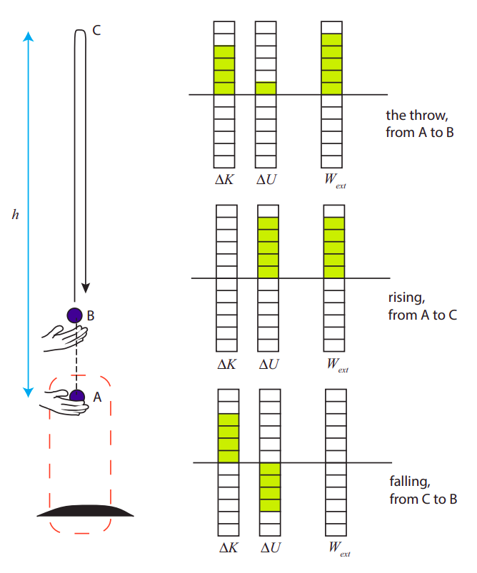
So how much work did you actually do? If we knew the distance from A to B, and the magnitude of the force you exerted, and if we could assume that your force was constant throughout, we could calculate \(W\) from the definition (10.2.5). But in this case, and many others like it, it is actually easier to find out how much total energy the system gained and just use Equation (\ref{eq:7.20}). To find \(\Delta E\) in practice, all we have to do is see how high the ball rises. At the ball’s maximum height (point C), as the second diagram shows, all the energy in the system is gravitational potential energy, and (as long as the system stays closed), all that energy is still equal to the work you did initially, so if the distance from A to C is \(h\) you must have done an amount of work
\[ W_{y o u}=\Delta U^{G}=m g h \label{eq:7.22} .\]
The third diagram in Figure \(\PageIndex{1}\) shows the work-energy balance for another time interval, during which the ball falls from C to B. Over this time, no external forces act on the ball (recall we have taken the system to be the ball and the earth, so gravity is an internal force). Then, the work done by the external forces is zero, and the change in the total energy of the system is also zero. The diagram just shows an increase in kinetic energy at the expense of an equal decrease in potential energy.
What about the work done by the internal forces? Equation (\ref{eq:7.18}) tells us that this work is equal to the negative of the change in potential energy. In this case, the internal force is gravity, and the corresponding energy is gravitational potential energy. This change in potential energy is clearly visible in all the diagrams; however, when you add to it the change in kinetic energy, the result is always equal to the work done by the external force only. Put otherwise, the internal forces do not change the system’s total energy, they just “redistribute” it among different kinds—as in, for instance, the last diagram in Figure \(\PageIndex{1}\), where you can clearly see that gravity is causing the kinetic energy of the system to increase at the expense of the potential energy.
We will use diagrams like the ones in Figure \(\PageIndex{1}\) to look at the work-energy balance for different systems. The idea is that the sum of all the columns on the left (the change in the system’s total energy) has to equal the result on the far-right column (the work done by the net external force): that is the content of the theorem (\ref{eq:7.20}). Note that, unlike the energy diagrams we used in Chapter 5, these columns represent changes in the energy, so they could be positive or negative.
Just as for the earlier energy diagrams, the picture we get will be different, even for the same physical situation, depending on the choice of system. This is illustrated in Figure \(\PageIndex{2}\) below, where I have taken the same throw shown in Figure \(\PageIndex{1}\), but now the system I’m looking at is the ball only. This means gravity is now an external force, as is the force of the hand, and the ball only has kinetic energy. Normally one would show the sum of the work done by the two external forces on a single column, but here I have chosen to break it up into two columns for clarity.
As you can see, during the throw the hand does positive work, whereas gravity does a comparatively small amount of negative work, and the change in kinetic energy is the sum of the two. For the longer interval from A to C (second diagram), gravity continues to do negative work until all the kinetic energy of the ball is gone. For the interval from C to B, the only external force is gravity, which now does positive work, equal to the increase in the ball’s kinetic energy.
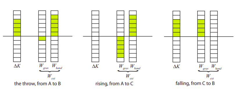
Of course, the numerical value of the actual work done by any particular force does not depend on our choice of system: in each case, gravity does the same amount of work in the processes illustrated in Figure \(\PageIndex{2}\) as in those illustrated in Figure \(\PageIndex{1}\). The difference, however, is that for the system in Figure \(\PageIndex{2}\), gravity is an external force, and now the work it does actually changes the system’s total energy, because the gravitational potential energy is now not included in that total.
Formally, it works like this: in the case shown in Figure \(\PageIndex{1}\), where the system is the ball and the earth, we have \(\Delta K + \Delta U^G = W_{hand}\). By the result (\ref{eq:7.18}), however, we have \(\Delta U^G = −W_{grav}\), and so this equation can be rearranged to read \(\Delta K = W_{grav} + W_{hand}\), which is just the result (\ref{eq:7.20}) when the system is the ball alone.
Ultimately, the reason we emphasize the importance of the choice of system is to prevent double counting: if you want to count the work done by gravity as contributing to the change in the system’s total energy, it means that you are, implicitly, treating gravity as an external force, and therefore your system must be something that does not have, by itself, gravitational potential energy (the case of the ball in Figure \(\PageIndex{2}\)); conversely, if you insist on counting gravitational potential energy as contributing to the system’s total energy, then you must treat gravity as an internal force, and leave it out of the calculation of the work done on the system by the external forces, which are the only ones that can change the system’s total energy.
The General Case- Systems With Dissipation
We are now ready to consider what happens when some of the internal interactions in a system are not conservative. There are two key observations to keep in mind: first, of course, that energy will always be conserved in a closed system, regardless of whether the internal forces are “conservative” or not: if they are not, it merely means that they will convert some of the “organized,” mechanical energy, into disorganized (primarily thermal) energy.
The second observation is that the work done by an external force on a system does not depend on where the force comes from—that is to say, what physical arrangement we use to produce the force. Only the value of the force at each step and the displacement of the point of application are involved in the definition (10.2.5). This means, in particular, that we can use a conservative interaction to do the work for us. It turns out, then, that the generalization of the result (\ref{eq:7.20}) to apply to all sorts of interactions becomes straightforward.
To see the idea, consider, for example, the situation in Figure \(\PageIndex{3}\) below. Here I have broken it up into two systems. System A, outlined in blue, consists of block 1 and the surface on which it slides, and includes a dissipative interaction—namely, kinetic friction—between the block and the surface. The force doing work on this system is the tension force from the rope, \(\vec F^t_{r,1}\).
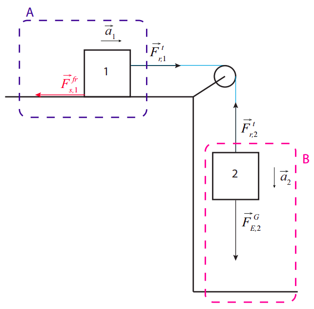
Because the rope is assumed to have negligible mass, this force is the same in magnitude as the force \(\vec F^t_{r,2}\) that is doing negative work on system B. System B, outlined in magenta, consists of block 2 and the earth and thus it includes only one internal interaction, namely gravity, which is conservative. This means that we can immediately apply the theorem (\ref{eq:7.20}) to it, and conclude that the work done on B by \(\vec F^t_{r,2}\) is equal to the change in system B’s total energy:
\[ W_{r, B}=\Delta E_{B} \label{eq:7.23} .\]
However, since the rope is inextensible, the two blocks move the same distance in the same time, and the force exerted on each by the rope is the same in magnitude, so the work done by the rope on system A is equal in magnitude but opposite in sign to the work it does on system B:
\[ W_{r, A}=-W_{r, B}=-\Delta E_{B} \label{eq:7.24} .\]
Now consider the total system formed by A+B. Assuming it is a closed system, its total energy must be constant, and so any change in the total energy of B must be equal and opposite the corresponding change in the total energy of A: \(\Delta E_B = −\Delta E_A\). Therefore,
\[ W_{r, A}=-\Delta E_{B}=\Delta E_{A} \label{eq:7.25} .\]
So we conclude that the work done by the external force on system A must be equal to the total change in system A’s energy. In other words, Equation (\ref{eq:7.20}) applies to system A as well, as it does to system B, even though the interaction between the parts that make up system A is dissipative.
Although I have shown this to be true just for one specific example, the argument is quite general: if I use a conservative system B to do some work on another system A, two things happen: first, by virtue of (\ref{eq:7.20}), the work done by B comes at the expense of its total energy, so \(W_{ext,A} = −\Delta E_B\). Second, if A and B together form a closed system, the change in A’s energy must be equal and opposite the change in B’s energy, so \(\Delta E_A = −\Delta E_B = W_{ext,A}\). So the result (\ref{eq:7.20}) holds for A, regardless of whether its internal interactions are conservative or not.
What is essential in the above reasoning is that A and B together should form a closed system, that is, one that does not exchange energy with its environment. It is very important, therefore, if we want to apply the theorem (\ref{eq:7.20}) to a general system—that is, one that includes dissipative interactions—that we draw the boundary of the system in such a way as to ensure that no dissipation is happening at the boundary. For example, in the situation illustrated in Figure \(\PageIndex{3}\), if we want the result (\ref{eq:7.25}) to apply we must take system A to include both block 1 and the surface on which it slides. The reason for this is that the energy “dissipated” by kinetic friction when two objects rub together goes into both objects. So, as the block slides, kinetic friction is converting some of its kinetic energy into thermal energy, but not all this thermal energy stays inside block 1. Put otherwise, in the presence of friction, block 1 by itself is not a closed system: it is “leaking” energy to the surface. On the other hand, when you include (enough of) the surface in the system, you can be sure to have “caught” all the dissipated energy, and the result (\ref{eq:7.20}) applies.
Energy Dissipated by Kinetic Friction
In the situation illustrated in Figure \(\PageIndex{3}\), we might calculate the energy dissipated by kinetic friction by indirect means. For instance, we can use the fact that the energy of system A is of two kinds, kinetic and “dissipated,” and therefore, by theorem (\ref{eq:7.20}), we have
\[\Delta K+\Delta E_{d i s s}=F_{r, 1}^{t} \Delta x_{1} \label{eq:7.26} .\]
Back in section 6.3, we used Newton’s laws to solve for the acceleration of this system and the tension in the rope; using those results, we can calculate the displacement \(\Delta x_1\) over any time interval, and the corresponding change in \(K\), and then we can solve Equation (\ref{eq:7.26}) for \(\Delta E_{diss}\).
If we do this, we will find out that, in fact, the following result holds,
\[ \Delta E_{d i s s}=-F_{s, 1}^{k} \Delta x_{1} \label{eq:7.27} \]
where \(F^k_{s,1}\) is the force of kinetic friction exerted by the surface on block 1, and must be understood to be negative in this equation (so that \(\Delta E_{diss}\) will come out positive, as it must be).
It is tempting to think of the product \(F^k_{s,1}\Delta x\) as the work done by the force of kinetic friction on the block, and most of the time there is nothing wrong with that, but it is important to realize that the “point of application” of the friction force is not a single point: rather, the force is “distributed,” that is to say, spread over the whole contact area between the block and the surface. As a consequence of this, a more general expression for the energy dissipated by kinetic friction between an object \(o\) and a surface \(s\) should be
\[ \Delta E_{\text {diss}}=\left|F_{s, o}^{k} \| \Delta x_{s o}\right| \label{eq:7.28} \]
where we are using the subscript notation \(x_{AB}\) to refer to “the position of B in the frame of A” (or “relative to A”); in other words, \(\Delta x_{so}\) is the change in the position of the object relative to the surface or, more simply, the distance that the object and the surface slip past each other (while rubbing against each other, and hence dissipating energy). If the surfaces is at rest (relative to the Earth), \(\Delta x_{so}\) reduces to \(\Delta x_{Eo}\), the displacement of the object in the Earth reference frame, and we can remove the subscript \(E\), as we typically do, for simplicity; however, in the rare cases when both the surface and the objet are moving what matters is how far they move relative to each other. In that case we have \( \left|\Delta x_{s o}\right|=\left|\Delta x_{o}-\Delta x_{s}\right| \) (with both \(\Delta x_o\) and \(\Delta x_s\) measured in the Earth reference frame).