
13.6: Kepler's Laws of Planetary Motion
- Page ID
- 46018

\( \newcommand{\vecs}[1]{\overset { \scriptstyle \rightharpoonup} {\mathbf{#1}} } \)
\( \newcommand{\vecd}[1]{\overset{-\!-\!\rightharpoonup}{\vphantom{a}\smash {#1}}} \)
\( \newcommand{\dsum}{\displaystyle\sum\limits} \)
\( \newcommand{\dint}{\displaystyle\int\limits} \)
\( \newcommand{\dlim}{\displaystyle\lim\limits} \)
\( \newcommand{\id}{\mathrm{id}}\) \( \newcommand{\Span}{\mathrm{span}}\)
( \newcommand{\kernel}{\mathrm{null}\,}\) \( \newcommand{\range}{\mathrm{range}\,}\)
\( \newcommand{\RealPart}{\mathrm{Re}}\) \( \newcommand{\ImaginaryPart}{\mathrm{Im}}\)
\( \newcommand{\Argument}{\mathrm{Arg}}\) \( \newcommand{\norm}[1]{\| #1 \|}\)
\( \newcommand{\inner}[2]{\langle #1, #2 \rangle}\)
\( \newcommand{\Span}{\mathrm{span}}\)
\( \newcommand{\id}{\mathrm{id}}\)
\( \newcommand{\Span}{\mathrm{span}}\)
\( \newcommand{\kernel}{\mathrm{null}\,}\)
\( \newcommand{\range}{\mathrm{range}\,}\)
\( \newcommand{\RealPart}{\mathrm{Re}}\)
\( \newcommand{\ImaginaryPart}{\mathrm{Im}}\)
\( \newcommand{\Argument}{\mathrm{Arg}}\)
\( \newcommand{\norm}[1]{\| #1 \|}\)
\( \newcommand{\inner}[2]{\langle #1, #2 \rangle}\)
\( \newcommand{\Span}{\mathrm{span}}\) \( \newcommand{\AA}{\unicode[.8,0]{x212B}}\)
\( \newcommand{\vectorA}[1]{\vec{#1}} % arrow\)
\( \newcommand{\vectorAt}[1]{\vec{\text{#1}}} % arrow\)
\( \newcommand{\vectorB}[1]{\overset { \scriptstyle \rightharpoonup} {\mathbf{#1}} } \)
\( \newcommand{\vectorC}[1]{\textbf{#1}} \)
\( \newcommand{\vectorD}[1]{\overrightarrow{#1}} \)
\( \newcommand{\vectorDt}[1]{\overrightarrow{\text{#1}}} \)
\( \newcommand{\vectE}[1]{\overset{-\!-\!\rightharpoonup}{\vphantom{a}\smash{\mathbf {#1}}}} \)
\( \newcommand{\vecs}[1]{\overset { \scriptstyle \rightharpoonup} {\mathbf{#1}} } \)
\(\newcommand{\longvect}{\overrightarrow}\)
\( \newcommand{\vecd}[1]{\overset{-\!-\!\rightharpoonup}{\vphantom{a}\smash {#1}}} \)
\(\newcommand{\avec}{\mathbf a}\) \(\newcommand{\bvec}{\mathbf b}\) \(\newcommand{\cvec}{\mathbf c}\) \(\newcommand{\dvec}{\mathbf d}\) \(\newcommand{\dtil}{\widetilde{\mathbf d}}\) \(\newcommand{\evec}{\mathbf e}\) \(\newcommand{\fvec}{\mathbf f}\) \(\newcommand{\nvec}{\mathbf n}\) \(\newcommand{\pvec}{\mathbf p}\) \(\newcommand{\qvec}{\mathbf q}\) \(\newcommand{\svec}{\mathbf s}\) \(\newcommand{\tvec}{\mathbf t}\) \(\newcommand{\uvec}{\mathbf u}\) \(\newcommand{\vvec}{\mathbf v}\) \(\newcommand{\wvec}{\mathbf w}\) \(\newcommand{\xvec}{\mathbf x}\) \(\newcommand{\yvec}{\mathbf y}\) \(\newcommand{\zvec}{\mathbf z}\) \(\newcommand{\rvec}{\mathbf r}\) \(\newcommand{\mvec}{\mathbf m}\) \(\newcommand{\zerovec}{\mathbf 0}\) \(\newcommand{\onevec}{\mathbf 1}\) \(\newcommand{\real}{\mathbb R}\) \(\newcommand{\twovec}[2]{\left[\begin{array}{r}#1 \\ #2 \end{array}\right]}\) \(\newcommand{\ctwovec}[2]{\left[\begin{array}{c}#1 \\ #2 \end{array}\right]}\) \(\newcommand{\threevec}[3]{\left[\begin{array}{r}#1 \\ #2 \\ #3 \end{array}\right]}\) \(\newcommand{\cthreevec}[3]{\left[\begin{array}{c}#1 \\ #2 \\ #3 \end{array}\right]}\) \(\newcommand{\fourvec}[4]{\left[\begin{array}{r}#1 \\ #2 \\ #3 \\ #4 \end{array}\right]}\) \(\newcommand{\cfourvec}[4]{\left[\begin{array}{c}#1 \\ #2 \\ #3 \\ #4 \end{array}\right]}\) \(\newcommand{\fivevec}[5]{\left[\begin{array}{r}#1 \\ #2 \\ #3 \\ #4 \\ #5 \\ \end{array}\right]}\) \(\newcommand{\cfivevec}[5]{\left[\begin{array}{c}#1 \\ #2 \\ #3 \\ #4 \\ #5 \\ \end{array}\right]}\) \(\newcommand{\mattwo}[4]{\left[\begin{array}{rr}#1 \amp #2 \\ #3 \amp #4 \\ \end{array}\right]}\) \(\newcommand{\laspan}[1]{\text{Span}\{#1\}}\) \(\newcommand{\bcal}{\cal B}\) \(\newcommand{\ccal}{\cal C}\) \(\newcommand{\scal}{\cal S}\) \(\newcommand{\wcal}{\cal W}\) \(\newcommand{\ecal}{\cal E}\) \(\newcommand{\coords}[2]{\left\{#1\right\}_{#2}}\) \(\newcommand{\gray}[1]{\color{gray}{#1}}\) \(\newcommand{\lgray}[1]{\color{lightgray}{#1}}\) \(\newcommand{\rank}{\operatorname{rank}}\) \(\newcommand{\row}{\text{Row}}\) \(\newcommand{\col}{\text{Col}}\) \(\renewcommand{\row}{\text{Row}}\) \(\newcommand{\nul}{\text{Nul}}\) \(\newcommand{\var}{\text{Var}}\) \(\newcommand{\corr}{\text{corr}}\) \(\newcommand{\len}[1]{\left|#1\right|}\) \(\newcommand{\bbar}{\overline{\bvec}}\) \(\newcommand{\bhat}{\widehat{\bvec}}\) \(\newcommand{\bperp}{\bvec^\perp}\) \(\newcommand{\xhat}{\widehat{\xvec}}\) \(\newcommand{\vhat}{\widehat{\vvec}}\) \(\newcommand{\uhat}{\widehat{\uvec}}\) \(\newcommand{\what}{\widehat{\wvec}}\) \(\newcommand{\Sighat}{\widehat{\Sigma}}\) \(\newcommand{\lt}{<}\) \(\newcommand{\gt}{>}\) \(\newcommand{\amp}{&}\) \(\definecolor{fillinmathshade}{gray}{0.9}\)- Describe the conic sections and how they relate to orbital motion
- Describe how orbital velocity is related to conservation of angular momentum
- Determine the period of an elliptical orbit from its major axis
Using the precise data collected by Tycho Brahe, Johannes Kepler carefully analyzed the positions in the sky of all the known planets and the Moon, plotting their positions at regular intervals of time. From this analysis, he formulated three laws, which we address in this section.
Kepler’s First Law
The prevailing view during the time of Kepler was that all planetary orbits were circular. The data for Mars presented the greatest challenge to this view and that eventually encouraged Kepler to give up the popular idea. Kepler’s first law states that every planet moves along an ellipse, with the Sun located at a focus of the ellipse. An ellipse is defined as the set of all points such that the sum of the distance from each point to two foci is a constant. Figure \(\PageIndex{1}\) shows an ellipse and describes a simple way to create it.
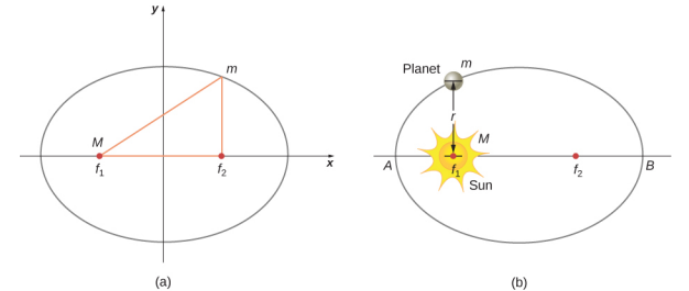
For elliptical orbits, the point of closest approach of a planet to the Sun is called the perihelion. It is labeled point A in Figure \(\PageIndex{1}\). The farthest point is the aphelion and is labeled point B in the figure. For the Moon’s orbit about Earth, those points are called the perigee and apogee, respectively.
An ellipse has several mathematical forms, but all are a specific case of the more general equation for conic sections. There are four different conic sections, all given by the equation
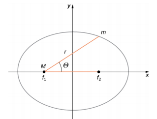
\[\frac{\alpha}{r} = 1 + e \cos \theta \ldotp \label{13.10}\]
The variables \(r\) and \(\theta\) are shown in Figure \(\PageIndex{2}\) in the case of an ellipse. The constants α and e are determined by the total energy and angular momentum of the satellite at a given point. The constant e is called the eccentricity. The values of \(\alpha\) and e determine which of the four conic sections represents the path of the satellite.
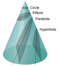
One of the real triumphs of Newton’s law of universal gravitation, with the force proportional to the inverse of the distance squared, is that when it is combined with his second law, the solution for the path of any satellite is a conic section. Every path taken by m is one of the four conic sections: a circle or an ellipse for bound or closed orbits, or a parabola or hyperbola for unbounded or open orbits. These conic sections are shown in Figure \(\PageIndex{3}\).
If the total energy is negative, then 0 ≤ e < 1, and Equation \ref{13.10} represents a bound or closed orbit of either an ellipse or a circle, where e = 0. [You can see from Equation 13.10 that for e = 0, r = \(\alpha\), and hence the radius is constant.] For ellipses, the eccentricity is related to how oblong the ellipse appears. A circle has zero eccentricity, whereas a very long, drawn-out ellipse has an eccentricity near one.
If the total energy is exactly zero, then e = 1 and the path is a parabola. Recall that a satellite with zero total energy has exactly the escape velocity. (The parabola is formed only by slicing the cone parallel to the tangent line along the surface.) Finally, if the total energy is positive, then e > 1 and the path is a hyperbola. These last two paths represent unbounded orbits, where m passes by M once and only once. This situation has been observed for several comets that approach the Sun and then travel away, never to return.
We have confined ourselves to the case in which the smaller mass (planet) orbits a much larger, and hence stationary, mass (Sun), but Equation 13.10 also applies to any two gravitationally interacting masses. Each mass traces out the exact sameshaped conic section as the other. That shape is determined by the total energy and angular momentum of the system, with the center of mass of the system located at the focus. The ratio of the dimensions of the two paths is the inverse of the ratio of their masses.
You can see an animation of two interacting objects at the My Solar System page at PhET. Choose the Sun and Planet preset option. You can also view the more complicated multiple body problems as well. You may find the actual path of the Moon quite surprising, yet is obeying Newton’s simple laws of motion.
Orbital Transfers
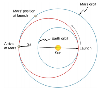
People have imagined traveling to the other planets of our solar system since they were discovered. But how can we best do this? The most efficient method was discovered in 1925 by Walter Hohmann, inspired by a popular science fiction novel of that time. The method is now called a Hohmann transfer. For the case of traveling between two circular orbits, the transfer is along a “transfer” ellipse that perfectly intercepts those orbits at the aphelion and perihelion of the ellipse. Figure \(\PageIndex{4}\) shows the case for a trip from Earth’s orbit to that of Mars. As before, the Sun is at the focus of the ellipse.
For any ellipse, the semi-major axis is defined as one-half the sum of the perihelion and the aphelion. In Figure \(\PageIndex{4}\), the semi-major axis is the distance from the origin to either side of the ellipse along the x-axis, or just one-half the longest axis (called the major axis). Hence, to travel from one circular orbit of radius r1 to another circular orbit of radius r2, the aphelion of the transfer ellipse will be equal to the value of the larger orbit, while the perihelion will be the smaller orbit. The semi-major axis, denoted a, is therefore given by \(a = \frac{1}{2} (r_{1} + r_{2})\).
Let’s take the case of traveling from Earth to Mars. For the moment, we ignore the planets and assume we are alone in Earth’s orbit and wish to move to Mars’ orbit. From Equation 13.9, the expression for total energy, we can see that the total energy for a spacecraft in the larger orbit (Mars) is greater (less negative) than that for the smaller orbit (Earth). To move onto the transfer ellipse from Earth’s orbit, we will need to increase our kinetic energy, that is, we need a velocity boost. The most efficient method is a very quick acceleration along the circular orbital path, which is also along the path of the ellipse at that point. (In fact, the acceleration should be instantaneous, such that the circular and elliptical orbits are congruent during the acceleration. In practice, the finite acceleration is short enough that the difference is not a significant consideration.) Once you have arrived at Mars orbit, you will need another velocity boost to move into that orbit, or you will stay on the elliptical orbit and simply fall back to perihelion where you started. For the return trip, you simply reverse the process with a retro-boost at each transfer point.
To make the move onto the transfer ellipse and then off again, we need to know each circular orbit velocity and the transfer orbit velocities at perihelion and aphelion. The velocity boost required is simply the difference between the circular orbit velocity and the elliptical orbit velocity at each point. We can find the circular orbital velocities from Equation 13.7. To determine the velocities for the ellipse, we state without proof (as it is beyond the scope of this course) that total energy for an elliptical orbit is
\[E = - \frac{GmM_{S}}{2a}\]
where MS is the mass of the Sun and a is the semi-major axis. Remarkably, this is the same as Equation 13.9 for circular orbits, but with the value of the semi-major axis replacing the orbital radius. Since we know the potential energy from Equation 13.4, we can find the kinetic energy and hence the velocity needed for each point on the ellipse. We leave it as a challenge problem to find those transfer velocities for an Earth-to-Mars trip.
We end this discussion by pointing out a few important details. First, we have not accounted for the gravitational potential energy due to Earth and Mars, or the mechanics of landing on Mars. In practice, that must be part of the calculations. Second, timing is everything. You do not want to arrive at the orbit of Mars to find out it isn’t there. We must leave Earth at precisely the correct time such that Mars will be at the aphelion of our transfer ellipse just as we arrive. That opportunity comes about every 2 years. And returning requires correct timing as well. The total trip would take just under 3 years! There are other options that provide for a faster transit, including a gravity assist flyby of Venus. But these other options come with an additional cost in energy and danger to the astronauts.
Visit this site (https://openstaxcollege.org/l/21plantripmars) for more details about planning a trip to Mars.
Kepler's Second Law
Kepler’s second law states that a planet sweeps out equal areas in equal times, that is, the area divided by time, called the areal velocity, is constant. Consider Figure \(\PageIndex{5}\). The time it takes a planet to move from position A to B, sweeping out area A1, is exactly the time taken to move from position C to D, sweeping area A2, and to move from E to F, sweeping out area A3. These areas are the same: A1 = A2 = A3.
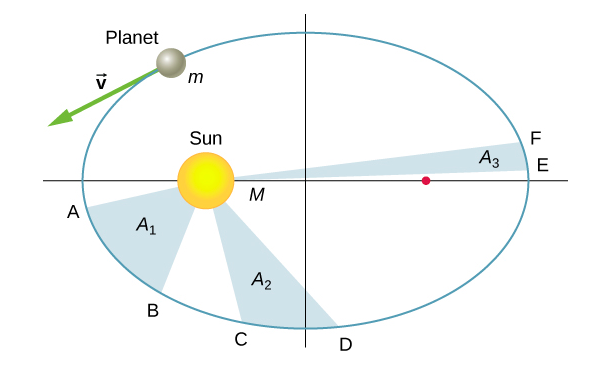
Comparing the areas in the figure and the distance traveled along the ellipse in each case, we can see that in order for the areas to be equal, the planet must speed up as it gets closer to the Sun and slow down as it moves away. This behavior is completely consistent with our conservation equation, Equation \ref{13.5}. But we will show that Kepler’s second law is actually a consequence of the conservation of angular momentum, which holds for any system with only radial forces.
Recall the definition of angular momentum from Angular Momentum, \(\vec{L} = \vec{r} \times \vec{p}\). For the case of orbiting motion, \(\vec{L}\) is the angular momentum of the planet about the Sun, \(\vec{r}\) is the position vector of the planet measured from the Sun, and \(\vec{p}\) = m\(\vec{v}\) is the instantaneous linear momentum at any point in the orbit. Since the planet moves along the ellipse, \(\vec{p}\) is always tangent to the ellipse.
We can resolve the linear momentum into two components: a radial component \(\vec{p}_{rad}\) along the line to the Sun, and a component \(\vec{p}_{perp}\) perpendicular to \(\vec{r}\). The cross product for angular momentum can then be written as
\[\begin{align*} \vec{L} &= \vec{r} \times \vec{p} \\[4pt] &= \vec{r} \times (\vec{p}_{rad} + \vec{p}_{perp}) \\[4pt] &= \vec{r} \times \vec{p}_{rad} + \vec{r} \times \vec{p}_{perp} \ldotp \end{align*}\]
The first term on the right is zero because \(\vec{r}\) is parallel to \(\vec{p}_{rad}\), and in the second term \(\vec{r}\) is perpendicular to \(\vec{p}_{perp}\), so the magnitude of the cross product reduces to
\[L = rp_{perp} = rmv_{perp}.\]
Note that the angular momentum does not depend upon \(p_{rad}\). Since the gravitational force is only in the radial direction, it can change only \(p_{rad}\) and not \(p_{perp}\); hence, the angular momentum must remain constant.
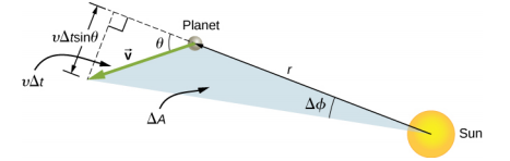
Now consider Figure \(\PageIndex{6}\). A small triangular area \(\Delta A\) is swept out in time \(\Delta t\). The velocity is along the path and it makes an angle \(\theta\) with the radial direction. Hence, the perpendicular velocity is given by \(v_{perp}= v\sin \theta\). The planet moves a distance \(\Delta\)s = v\(\Delta\)tsin\(\theta\) projected along the direction perpendicular to \(r\). Since the area of a triangle is one-half the base (\(r\)) times the height (\(\Delta s\)), for a small displacement, the area is given by
\[\Delta A = \frac{1}{2} r \Delta s. \nonumber\]
Substituting for \(\Delta s\), multiplying by \(m\) in the numerator and denominator, and rearranging, we obtain
\[\Delta A = \frac{1}{2} r \Delta s = \frac{1}{2} r (v \Delta t \sin \theta) = \frac{1}{2m} r (mv \sin \theta \Delta t) = \frac{1}{2m} r (mv_{perp} \Delta t) = \frac{L}{2m} \Delta t \ldotp\]
The areal velocity is simply the rate of change of area with time, so we have
\[ \text{areal velocity} = \frac{\Delta A}{\Delta t} = \frac{L}{2m} \ldotp\]
Since the angular momentum is constant, the areal velocity must also be constant. This is exactly Kepler’s second law. As with Kepler’s first law, Newton showed it was a natural consequence of his law of gravitation.
You can view an animated version of Figure \(\PageIndex{6}\), and many other interesting animations as well, at the School of Physics (University of New South Wales) site.
Kepler's Third Law
Kepler’s third law states that the square of the period is proportional to the cube of the semi-major axis of the orbit. In Satellite Orbits and Energy, we derived Kepler’s third law for the special case of a circular orbit. Equation \ref{13.8} gives us the period of a circular orbit of radius r about Earth:
\[T = 2 \pi \sqrt{\frac{r^{3}}{GM_{E}}} \ldotp \label{13.5.5}\]
For an ellipse, recall that the semi-major axis is one-half the sum of the perihelion and the aphelion. For a circular orbit, the semi-major axis (\(a\)) is the same as the radius for the orbit. In fact, Equation \ref{13.5.5} gives us Kepler’s third law if we simply replace \(r\) with \(a\) and square both sides.
\[T^{2} = \frac{4 \pi^{2}}{GM} a^{3} \label{13.11}\]
We have changed the mass of Earth to the more general \(M\), since this equation applies to satellites orbiting any large mass.
Determine the semi-major axis of the orbit of Halley’s comet, given that it arrives at perihelion every 75.3 years. If the perihelion is 0.586 AU, what is the aphelion?
Strategy
We are given the period, so we can rearrange Equation \ref{13.11}, solving for the semi-major axis. Since we know the value for the perihelion, we can use the definition of the semi-major axis, given earlier in this section, to find the aphelion. We note that 1 Astronomical Unit (AU) is the average radius of Earth’s orbit and is defined to be 1 AU = 1.50 x 10¹¹ m.
Solution
Rearranging Equation \ref{13.11} and inserting the values of the period of Halley’s comet and the mass of the Sun, we have
\[\begin{split} a & = \left(\dfrac{GM}{4 \pi^{2}} T^{2}\right)^{1/3} \\ & = \left(\dfrac{(6.67 \times 10^{-11}\; N\; \cdotp m^{2}/kg^{2})(2.00 \times 10^{30}\; kg)}{4 \pi^{2}} (75.3\; yr \times 365\; days/yr \times 24\; hr/day \times 3600\; s/hr)^{2}\right)^{1/3} \ldotp \end{split}\]
This yields a value of 2.67 x 10¹² m or 17.8 AU for the semi-major axis. The semi-major axis is one-half the sum of the aphelion and perihelion, so we have
\[\begin{split} a & = \frac{1}{2} (aphelion + perihelion) \\ aphelion & = 2a - perihelion \ldotp \end{split}\]
Substituting for the values, we found for the semi-major axis and the value given for the perihelion, we find the value of the aphelion to be 35.0 AU.
Significance
Edmond Halley, a contemporary of Newton, first suspected that three comets, reported in 1531, 1607, and 1682, were actually the same comet. Before Tycho Brahe made measurements of comets, it was believed that they were one-time events, perhaps disturbances in the atmosphere, and that they were not affected by the Sun. Halley used Newton’s new mechanics to predict his namesake comet’s return in 1758.
The nearly circular orbit of Saturn has an average radius of about 9.5 AU and has a period of 30 years, whereas Uranus averages about 19 AU and has a period of 84 years. Is this consistent with our results for Halley’s comet?