29: Solving the Wave Equation with Fourier Transforms

[** This chapter is under construction **]

In the next chapter we will introduce the wave equation due to its importance in understanding the dynamics of the primordial plasma. In one dimension the wave equation can be written as 

\[\frac{\partial^2 \Psi (x, t)} { \partial t^2} = v^2 \frac{\partial^2 \Psi (x, t)} {\partial x^2}. \label{eqn:wave}\]

We will leave a discussion of the physics of this equation and the primordial plasma to the next chapter. Here, we will focus on the use of Fourier methods to solve for the evolution of \( \Psi(x,t) \) assuming it obeys the above equation and that we are given the value of \(\Psi\) and its time derivative at some initial time for all values of \(x\). Fourier methods have a broad range of applications in physics. They have utility well beyond the dynamics of the wave equation in both experimental and theoretical physics. For the student of physics, time spent developing facility with Fourier transforms is time well spent.

Let's see what happens with an ansatz of the form
\[\Psi(x,t) = A(t) \cos(kx); \label{eqn:Ansatz1} \]
i.e., let's assume the wave has a fixed spatial pattern of a cosine of wavelength \(\lambda/(2\pi)\), with an amplitude that varies with time.

Plugging this ansatz in to Eq. \ref{eqn:wave} we find that it is a solution of Eq. \ref{eqn:wave} as long as
\[\ddot A(t) = -v^2k^2 A(t); \label{eqn:HO} \]
i.e., as long as \(A(t)\) obeys a harmonic oscillator equation.

Box: do the above plugging in to arrive at Eq. \ref{eqn:HO}.

Exercise \(\PageIndex{1}\)

Do the above "plugging in" to arrive at Eq. \ref{eqn:HO}

Answer

TBD

 

The general solution to Eq. \ref{eqn:HO} is
\[A(t) = \alpha \cos(kvt) + \beta \sin(kvt) \].
The constants \(\alpha\) and \(\beta\) can be determined from initial conditions \(A(0)\) and \(\dot A(0)\).

Because it will be helpful to see a specific solution, let's assume the ansatz Eq. \ref{eqn:Ansatz1}, set \(k = 2\pi/{\rm Mpc}\), \(A(0) = 1\) and \(\dot A(0) = 0\). Note that this means we have a wave of wavelength 1 Mpc that starts off at rest with unit amplitude. One can show that in this case \(\alpha = 1, \beta = 0\), and the solution for \(\Psi\) is therefore
\[\Psi(x,t) = \cos(kvt)\cos(kx) \label{eqn:SimpleSolution1}\]
where \(k = 2\pi/{\rm Mpc}\). This solution is graphed in the following animation:

            

Exercise \(\PageIndex{2}\)

Check that Eq. \ref{eqn:SimpleSolution1} satisfies the wave equation and is consistent with the given initial conditions.

Answer

TBD

We've seen a specific solution to the wave equation. We're now going to work our way toward a completely general solution, and a nifty solution method that relies on the properties we've just seen above for how a cosine (or sine, as we'll see) spatial pattern evolves over time.

Our general solution method will exploit the fact that any some of two solutions to the wave equation is itself a solution to the wave equation.

Exercise \(\PageIndex{3}\)

Show that if \(\Psi_1(x,t)\) and \(\Psi_2(x,t)\) are both solutions of Eq. \ref{eqn:wave} then \(\Psi_1(x,t) + \Psi_2(x,t)\) is a solution also.

Answer

TBD

Let's now introduce another particular solution to the wave equation, which we will need for the general solutions, and that is:
\[\Psi(x,t) = B(t)\sin(kx). \label{eqn:Ansatz2} \]

Exercise \(\PageIndex{4}\)

Show that Eq. \ref{eqn:Ansatz2} is indeed a solution of Eq. \ref{eqn:wave} as long as \(\ddot B = -k^2v^2 B\).

Answer

TBD

We are now ready to present the broad outlines of a solution strategy that takes advantage of the fact that any function of \(x\) can be written as a sum over cosines and sines of various wavelengths (an assertion that we will discuss more below). The basic idea is that the amplitudes of these sines and cosines will obey a HO equation, and so their time evolution is simple. The general solution is thus a sum over cosines and sines, each with their individual amplitude evolving harmonically at its particular rate.

To be more explicit, here, qualitatively, are the steps:

1) We can write any \(\Psi(x,t)\) as a sum over cosines and sines with different wavelengths (and hence different values of \(k\)):
\[\Psi(x,t) = A_1(t) \cos(k_1 x) + B_1(t) \sin(k_1 x)  + A_2(t) \cos(k_2 x) + B_2(t) \sin(k_2 x) + .... \label{eqn:GeneralSolution1}\]
2) If \(\Psi(x,t)\) obeys the wave equation then each of the time-dependent amplitudes obeys their own harmonic oscillator equation
\[\ddot A_n(t) = -k_n^2v^2 A(t) \ \ \ {\rm and} \ \ \ \ddot B_n(t) = -k_n^2 v^2 B(t). \]
3) These equations for the amplitudes are easy to solve , and their solutions are completely independent of one another: how \(A_3(t)\) evolves has no impact on how \(B_2(t)\) evolves, for example. (Note that this is kind of amazing because they are both waves in the same medium at the same time and location.)

4) With the time evolution of the amplitudes determined (using the given initial conditions), we can just plug those into Eq. \ref{eqn:GeneralSolution1} to get the solution.

One thing we have not told you yet is how one, in practice, actually writes out the terms on the right-hand side of Eq. \ref{eqn:GeneralSolution1}. For example, how does one know what values of \(k_1\) are needed? Also, how does one get the needed initial conditions for the \(A_n\) and \(B_n\)? We'll get to that, but for now let's look at an example of this solution method at work.

Let's work out how \(\Psi(x,t)\) will evolve if it starts off as a triangle wave at rest. Let's assume the triangle wave has a wavelength of 1 Mpc, initially has an amplitude of unity, is initially at rest (\(\dot\Psi(x,0)=0\)) and is phased so that it is zero at the origin (\(\Psi(0,0) = 0\)). Let's further assume it obeys the wave equation with speed \(v\); i.e. Eq. \ref{eqn:wave}.

We will state without proof here (but the proof is not difficult; see Wolfram Alpha)  that the initial configuration \(\Psi(x,0)\) can be written as
\[\Psi(x,0) = \Sigma_{n=1}^\infty \left(A_n(0) \cos(k_n x) + B_n(0) \sin(k_nx) \right)  \]
with \(A_n(0) = 0\) for all \(n\), \(B_n(0)= 0\) for even \(n\), and \(B_n(0) = 8/\pi^2 (-1)^{(n-1)/2}/n^2\) for odd \(n\) and their time derivatives at \(t=0\) vanishing. In the figure we show how well the triangle wave is approximated by the series as we increase the number of terms we are including in the sum, by increasing the maximum value of \(n\), so you can see that this series representation does indeed seem to work. In addition to the sum, we also show the individual terms.

**Lucas, please insert a still (non-animated) figure here showing the series converging**

To be able to explicitly show the solutions, and so this is not too cumbersome, we will restrict ourselves from here on out to just the first three terms in the sum. From the initial conditions written above we thus have
\[ \Psi(x,t) = \frac{8}{\pi^2}\cos\left(\frac{2\pi}{Mpc} vt\right) \sin\left(\frac{2\pi}{Mpc} x\right) - \frac{8}{9\pi^2}\cos\left(\frac{6\pi}{Mpc} vt\right) \sin\left(\frac{6\pi}{Mpc} x\right) + \frac{8}{25\pi^2}\cos\left(\frac{10\pi}{Mpc} vt\right) \sin\left(\frac{10\pi}{Mpc} x\right) + .... \]
The solution is illustrated in the animation.

**Lucas, please insert an animated figure here as described immediately above.**

**Lloyd: insert here some wrap-up of above section  **

The Continuous Fourier Transform

We just saw a solution for an initial spatial configuration with wavelength \(\lambda = 1\) Mpc which can be represented as a sum over sines and cosines (just sines in this case) with an (infinite) set of discrete \(k\) values, specifically \(k_n = 2n \pi/\lambda\). Note that the spacing between \(k\) values in this case is \(\Delta k = 2\pi/\lambda\). For the more general situation of a function of space that is not periodic, we can think of it is a periodic function with infinite wavelength. As the wavelength goes to infinity, the \(\Delta k\) goes to zero. So we see we need a continuum of values of \(k\). For the general case then we swap the sum over \(i\) with an integral over \(k\):
\[\Psi(x,t) = \int_0^\infty dk [A(k,t) \cos(kx) + B(k,t)\sin(kx)]. \label{eqn:InverseFTsinecosine}\]

It turns out there is a more compact way of working with this decomposition into cosines and sines if we use complex numbers. We can write instead
\[\Psi(x,t) = \int_{-\infty}^\infty dk \tilde \Psi(k,t)e^{ikx} \label{eqn:InverseFT}\]
which is a mathematical opertation known as the inverse Fourier transform. For \(\Psi(x,t)\) a real function, Eq. \ref{eqn:InverseFTsinecosine} and Eq. \ref{eqn:InverseFT} are equivalent if we make the identification
\[A(k,t) = 2 Re \tilde \Psi(k,t) \ \ \ {\rm and}\ \ \ B(k,t) = 2 Im \Psi(k,t) \]
for \( k> 0\) where "Re" and "Im" indicate taking the real and imaginary parts respectively. Homework problem TBD is to prove these relationships are true. 

 

Solving the Wave Equation in Fourier Space

You may already be familiar with a method for solving partial differential equations known as separation of variables. Using separation of variables to solve the wave equation, we would guess a solution of the form \( \Psi (x, t) = X(x)T(t) \). Plugging this into the wave equation yields two simple ODE's: one for \( T(t) \) and one for \( X(x) \). Now though, we'd like to introduce you to another way to analyze partial differential equations (PDE's): Fourier methods.

The basic idea here is that we transform from a basis in which the time evolution is complicated (one in which the field is described as a function of position), to a basis in which the time evolution is remarkably simple (one in which the field is described as a collection of Fourier modes). We do the time evolution in this new basis, and then we transform back to our original basis. 

We will use the discrete version of the Fourier transform here, as that is perhaps an easier starting point to wrap one's mind around first. We include a discussion of the continuous Fourier transform, which is easy to understand as the continuum limit of the discrete version. 

[To be done: all this needs to be translated to discrete from continuous and then we need to create a section on the continuum limit.]

We start off, in a manner that may seem a little backwards, by defining the inverse Fourier transformation: 

\[ h(x) = \frac{1}{2\pi}\int_{-\infty}^{\infty} dk e^{ikx} \tilde h(k).  \label{eqn:IFT} \]

The \(\tilde h(k)\) are complex (have real and imaginary parts) and recall that \(\exp(ikx) = \cos(kx)+i\sin(kx)\). We start here because there is a theorem that states that a broad class of functions of \(x\) can all be written as sums over \(\exp(ikx)\) for a continuum of values of \(k\), and for appropriately chosen complex coefficients of the \(\exp(ikx)\). That is, we can represent the information in a function \(h(x)\) by its Fourier coefficients \(\tilde h(k)\), with the relationship between the two given by Equation\ref{eqn:IFT}. The functions, \(\exp(ikx)\) are known as Fourier modes. Since \(\exp(ikx) = \exp(ik(x+2\pi/k))\) we see that a Fourier mode has a wavelength of \(2\pi/k\). We call \(k\) the 'wavenumber.' 

One can do Fourier transforms in time or in space or both. Here we are only going to be doing Fourier transforms in space, although we will consider Fourier transforms in space at all points in time. To be explicit about this, we can rewrite Equation  \ref{eqn:IFT} to include a \(t\) argument of the functions:

\[ h(x,t) = \frac{1}{2\pi}\int_{-\infty}^{\infty} dk e^{ikx} \tilde h(k,t).  \label{eqn:IFTwithTime} \]

It's the same transformation, but now we are explicit that we do this transformation at all values of \(t\). 

Recall that we claimed that the evolution of the \(\tilde h(k,t)\) would be simple. To figure out what equation governs the evolution of these coefficients, we need to know how to figure out for a given \(h(x,t)\) what is  \(\tilde h(k,t)\). But we are going to return to leaving off the \(t\) dependence, for simplicity. We already know how to go from \(\tilde h(k)\) to \(h(x)\), that is what we called the inverse Fourier transform, Equation  \ref{eqn:IFT}. So we are looking now for the inverse of this, what we will naturally call the Fourier transform. 

Let's work our way toward the Fourier transform by first pointing out  an important property of Fourier modes: they are orthonormal. This means that if we integrate over all space one Fourier mode, \(e^{-ikx}\), multiplied by the complex conjugate of another Fourier mode \(e^{ik'x}\) the result is \(2\pi\) times the Dirac delta function:

\[\int_{-\infty}^{\infty} dx e^{-ikx}e^{ik'x} = 2\pi \delta(k-k') \label{eqn:OrthoNormal}\]

where the Dirac delta function is a continuum version of the Kronecker delta function, defined by its integral over \(k\) such that

\[ \int_{-\infty}^{\infty} dk \delta(k-k') f(k) = f(k'). \label{eqn:DiracDelta} \]

You can loosely think of the Dirac delta function as being zero for all non-zero values of its argument and  \(+\infty\) when its argument is zero. 

From these equations one can derive what we call the Fourier transform:

\[ \tilde h(k) = \int_{-\infty}^{\infty} dx e^{-i kx} h(x) \label{eqn:FT} \]

and thus the answer to the question of how we deduced \(\tilde h(k,t)\) from \(h(x,t)\).

 

Box \(\PageIndex{6}\)

Exercise 27.1.1: Show that one can derive Equation \ref{eqn:FT} from Equations \ref{eqn:IFT}, \ref{eqn:OrthoNormal}, and \ref{eqn:DiracDelta}.

 

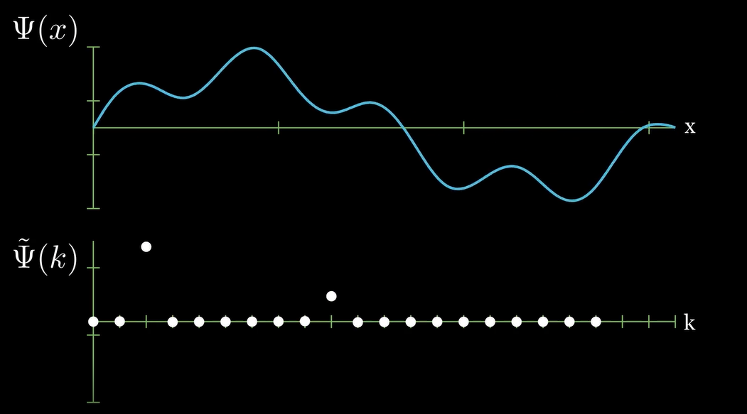
Before deriving the evolution equation for the Fourier coefficients, let's look at an example of a function in the position basis and what it looks like in the Fourier basis. The following image shows a wave on the top panel, \(\Psi(x)\), and the Fourier transform of that wave on the bottom panel. (Note that \( \mathcal{F}(\Psi) \) indicates the operation of Fourier transforming the function \( \Psi(x) \); i.e., \( \mathcal{F}(\Psi) = \tilde \Psi(k) \).  Notice how the Fourier transform 'picks out' the two spatial frequencies of which the wave is composed.

[Problem: this is a discreet FT and we have only talked about continuum.]

 

 

For a \(\Psi(x,t)\) that obeys the wave equation, let's now find the equation that its Fourier coefficients, \(\tilde \Psi(k,t)\), satisfy. Starting from the wave equation,

\[\frac{\partial^2 \Psi (x, t)} { \partial t^2} = v^2 \frac{\partial^2 \Psi (x, t)} {\partial x^2}, \]

and then substituting in the inverse Fourier transform \( \Psi(x,t) = \frac{1}{2\pi} \int_{- \infty} ^ {\infty} dk \tilde \Psi(k,t) e^{-ikx}  \) we find:

\[ \frac{ \partial^2 } { \partial t^2} \int_{- \infty} ^ {\infty} dk \tilde \Psi(k,t) e^{-ikx}  = v^2 \frac{ \partial^2 } { \partial x^2} \int_{- \infty} ^ {\infty} dk \tilde \Psi(k,t)  e^{-ikx} \]

Distributing the derivatives gives:

\[ \int_{- \infty} ^ {\infty}  dk \frac{ \partial^2 \tilde \Psi(k,t) e^{-ikx}}  { \partial t^2}  = - \int_{- \infty} ^ {\infty} dk (kv)^2  \tilde \Psi(k,t) e^{-ikx}.\]

We can then rearrange terms to find:

\[ \int_{- \infty} ^ {\infty} dk \bigg [ \frac{ \partial^2 \tilde \Psi(k,t)}   { \partial t^2}   + (kv)^2 \tilde \Psi(k,t) \bigg ] e^{-ikx} = 0. \]

It turns out that the only way the left-hand side can be zero for all values of \(x\) is if the quantity in square brackets is zero for all values of \(k\) (see Box below) so we get that

\[ \frac{ \partial^2 \tilde \Psi(k,t)}   { \partial t^2}   + (kv)^2 \tilde \Psi(k,t) = 0. \label{eqn:WaveEquationInFourierSpace}\]

 

Box \(\PageIndex{7}\)

Exercise 27.2.1: Prove that if

\[  \int_{- \infty} ^ {\infty} dk f(k) e^{-ikx} = 0 \label{eqn:IntegratesToZero}\] 

for all \(x\), then \(f(k) = 0\) for all \(k\). 

First, multiply the left-hand side of Equation \ref{eqn:IntegratesToZero}  by \(\exp(-ik'x)\), integrate it over all \(k'\), and identify the Dirac delta function to end up with:

\[ \frac{ \partial^2 \tilde \Psi(k')}   { \partial t^2}   + (k'v)^2 \tilde \Psi(k')  = 0. \] 

Finally, note that since this is true for all \(k'\) it's also true for all \(k\).

Equation \ref{eqn:WaveEquationInFourierSpace} is a very common differential equation. You've probably solved it many times! You may recognize it better if we let \( y = \tilde \Psi(k,t) \), so that it reads \( \ddot{y} + k^2 v^2 y = 0\). We can easily write down a solution:

\[   \tilde \Psi(k,t) = A(k) \sin{ (kvt) } + B(k) \cos{ (kvt) } . \]

Thus our general solution back in the space basis is 

\[\Psi(x,t) = \frac{1}{2\pi} \int_{-\infty}^{\infty} dk \bigg [ A(k) \sin{ (kvt) } + B(k) \cos{ (kvt) } \bigg ] e^{ikx}. \] 

We can find \(A(k)\) and \(B(k)\) if we know \(\Psi(x,t)\) and \(\dot \Psi(x,t)\) at \(t=0\) because 

\[\Psi(x,t=0) = \frac{1}{2\pi} \int_{-\infty}^{\infty} dk B(k)  e^{ikx} \]

and

\[\dot \Psi(x,t=0) = \frac{1}{2\pi}\int_{-\infty}^{\infty} dk kv A(k) e^{ikx} \].

Given these relationships we see that to get \(B(k)\) and \(A(k)\) we Fourier transform the initial value of \(\Psi\) and its time derivative:

\[ B(k) = \int_{-\infty}^{\infty} dx \Psi(x,t=0) e^{-ikx} \]

and

\[A(k) = \frac{1}{kv} \int_{-\infty}^{\infty} dx \dot \Psi(x,t=0) e^{-ikx}. \]

To summarize, we found that in a Fourier basis, rather than the original space basis, the wave equation simplifies from a partial differential equation to a set of uncoupled ordinary differential equations. The wave equation is easily solved in the Fourier basis and we provided the general solution. This general solution depends on two functions of \(k\) that can be derived from the initial conditions. 

Consider the following initial conditions on our string \( \Psi (x, t = 0) = \sin ( 2 x) \). This is a single wave with k = 2. Taking the Fourier transform, we find: \( \mathcal{F} \bigg ( \Psi (x, t = 0) \bigg ) = \delta (x - 2) \). The Fourier transform is 1 where k = 2 and 0 otherwise. We see that over time, the amplitude of this wave oscillates with cos(2 v t). The solution to the wave equation for these initial conditions is therefore \( \Psi (x, t) = \sin ( 2 x) \cos (2 v t) \). This wave and its Fourier transform are shown below. The power spectrum is merely the Fourier transform squared.

Now consider we have initial conditions which are more complicated, but can be written as an infinite sum of sine waves as follows:

\[ \Psi (x, t =0) = \sum_{i=1}^{\infty} A_i \sin (k_i  x) \]

Taking the Fourier transform, we find the following sum of delta functions:

\[ \mathcal{F} \bigg ( \Psi (x, t = 0) \bigg ) = \sum_{i = 1}^{\infty} A_i \delta (k- k_i) \]

Which oscillate in time according to:

\[ \mathcal{F} \bigg ( \Psi (x, t) \bigg ) = \sum_{i = 1}^{\infty} A_i \delta (k - k_i) \cos ( k_i v t) \]

Returning to real space we find:

\[ \Psi (x, t) = \sum_{i = 1}^{\infty} A_i \sin ( k_i x ) \cos ( k_i v t) \]

The takeaway here is that the solution to the wave equation can always be written as a sum of independent standing waves. Some examples are shown below. The top panel shows the wave and the bottom panel shows the Fourier transform of that wave. Notice how the evolution seems very complex in real space, but in Fourier space it is merely independent delta functions of oscillating amplitude. This is the beauty of using Fourier methods to analyze the wave equation. If you wanted to see the power spectrum, you would simply square the Fourier transform.

Exercise \(\PageIndex{8}\)

Consider the heat equation for a straight rod: \( \frac{d \Psi} {dt} = \alpha \frac{d^2 \Psi} {dt^2} \), where \( \Psi (x, t) \) is the temperature at a certain point on the beam. Using the techniques from the previous section, find the evolution of Fourier modes. How can this physically be interpreted?

Answer

We plug in the Fourier representation of \( \Psi \) into the heat equation: 

\( \frac{ d } { dt} \int_{- \infty} ^ {\infty}  \mathcal{F} ( \Psi) e^{-ikx} dk = \alpha \frac{ \partial^2 } { \partial x^2} \int_{- \infty} ^ {\infty}  \mathcal{F} ( \Psi)  e^{-ikx} dk \)

Distributing the derivatives and some algebra gives:

\( \int_{- \infty} ^ {\infty} \bigg [ \frac{ d \mathcal{F} (\Psi) }  { dt }  e^{-ikx} + \alpha k^2 e^{-ikx} \mathcal{F} ( \Psi) \bigg ] dk = 0 \)

Which is satisfied if:

\(  \frac{d \mathcal{F}(\Psi)} { dt} + \alpha  k^2\mathcal{F}( \Psi) = 0 \)

Using separation of variables, we find:

\( \mathcal{F}(\Psi) = C e^{-\alpha k^2 t} \), where C is a constant determined by initial conditions.

Therefore, we see that higher frequencies decay faster. This makes sense, as we would expect spikes in temperature (high curvature) to disappear quickly, whereas more smooth temperature gradients will decay more slowly.