
1.1: Overview


- Last updated
- Jan 3, 2025
- Save as PDF

( \newcommand{\kernel}{\mathrm{null}\,}\)
Cosmologists speak with a high degree of confidence about conditions that existed billions of years ago when the universe was quite different from how we find it today: 109 times hotter than today, over 1030 times denser, and much much smoother, with variations in density from one place to another only as large as one part in 100,000. We claim to know the composition of the universe at this early time, dominated almost entirely by thermal distributions of photons and subatomic particles called neutrinos. We know in detail many aspects of the evolutionary process that connects this early universe to the current one. Our models of this evolution have been highly predictive and enormously successful.
In this chapter we provide an overview of our subject, broken into two parts. The first is focused on the discovery of the expansion of the universe in 1929, and the theoretical context for this discovery, which is given by Einstein's general theory of relativity (GR). The second is on the implications of this expansion for the early history of the universe, and relics from that period observable today: the cosmic microwave background and the lightest chemical elements. The consistency of such observations with theoretical predictions is why we speak confidently about such early times, approximately 14 billion years in our past.
Overview Part I: The Expansion of Space and the Contents of the Universe
Space is not what you think it is. It can curve and it can expand over time. We can observe the consequences of this expansion over time, and from these observations infer some knowledge of the Universe's contents.
Newton-Maxwell Incompatibility and Einstein's Theory
It would be difficult to overstate the impact that Einstein’s 1915 General Theory of Relativity has had on the field of cosmology. So we begin our review with some discussion of the General Theory, and its origin in conflicts between Newtonian physics and Maxwell’s theory of electric and magnetic fields. We end our discussion of Einstein’s theory with its prediction that the universe must be either expanding or contracting.
Newton’s laws of motion and gravitation have amazing explanatory powers. Relatively simple laws describe, almost perfectly, the motions of the planets and the moon, as well as the motions of bodies here on Earth -- at least at speeds much lower than the speed of light. The discovery of the planet Neptune provides us with an example of their predictive power. The discovery began with calculations by Urbain Le Verrier. Using Newton’s theory, he was able to explain the observed motion of Uranus only if he posited the existence of a planet with a particular orbit, an extra planet beyond those known at the time. Without the gravitational pull of this not-yet-seen planet, Newton's theory could not account for the motion of Uranus. Following up on his prediction, made public in 1846, Johannes Gottfried Galle looked for a new planet where Le Verrier said it was to be found and, indeed, there it was, what we now call Neptune. The time from prediction to confirmation was less than a month.
Less than 20 years after the discovery of Neptune, a triumph of the Newtonian theory, came a great inductive synthesis: Maxwell’s theory of electric and magnetic fields. The experiments that led to this synthesis, and the synthesis itself, have enabled the development of a great range of technologies we now take for granted such as electric motors, radio, television, cellular communication networks and microwave ovens. More important for our subject, they also led to radical changes to our conception of space and time.
These radical changes arose from conflicts between the synthesis of Maxwell with that of Newton. For example, in the Newtonian theory velocities add: if A sees B move at speed v to the west, and B sees C moving at speed v to the west relative to B, then A sees C moving at speed v+v = 2v to the west. But one solution to the Maxwell equations is a propagating disturbance in the electromagnetic fields that travels with a fixed speed of about 300,000 km/sec. Without modification, the Maxwell equations predict that both A and B would see electromagnetic wave C moving away from them at a speed of 300,000 km/sec, violating the velocity addition rule that one can derive from Newtonian concepts of space and time.
Einstein’s solution to these inconsistencies includes an abandonment of Newtonian concepts of space and time. This abandonment, and discovery of the replacement principles consistent with the Maxwell theory, happened over a considerable amount of time. A solution valid in the absence of gravitation came out first in 1905, with Einstein’s paper titled (in translation from German) “On the Electrodynamics of Moving Bodies.” His effort to reconcile gravitational theory with Maxwell’s theory did not fully come together until November of 1915, with a series of lectures in Berlin where he presented his General Theory of Relativity.

One indicator that Einstein was on the right track was his realization, in September 1915, that his theory provided an explanation for a longstanding problem in solar system dynamics known as the anomalous perihelion precession of Mercury. Given Newtonian theory, and an absence of other planets, Mercury would orbit the Sun in an ellipse shape. However, the influence of the other planets is to make Mercury follow almost an ellipse, in a pattern that is well approximated as that of a slowly rotating ellipse. One way of expressing this rotation is to say how rapidly the location of closest approach, called perihelion, is rotating around the Sun. Mercury’s perihelion precession is quite slow. In fact, it’s less than one degree per century. More precisely, it’s 575 seconds of arc per century, where a second of arc is a degree divided by 3,600 (just as a second is an hour divided by 3,600).
Urbain Le Verrier, following his success with Neptune, took up the question of this motion of Mercury: could the perihelion precession be understood as resulting from the pulls on Mercury from the other planets. He found that he could ascribe about 532 seconds of arc to the other planets, but not the entire 575. There is an additional, unexplained (“anomalous”) precession of 43 seconds of arc per century. Le Verrier, of course, knew how to handle situations like this. He proposed that this motion is caused by a not-yet-discovered planet. This planet was proposed to have an orbit closer to the Sun than Mercury’s and eventually had the name Vulcan.
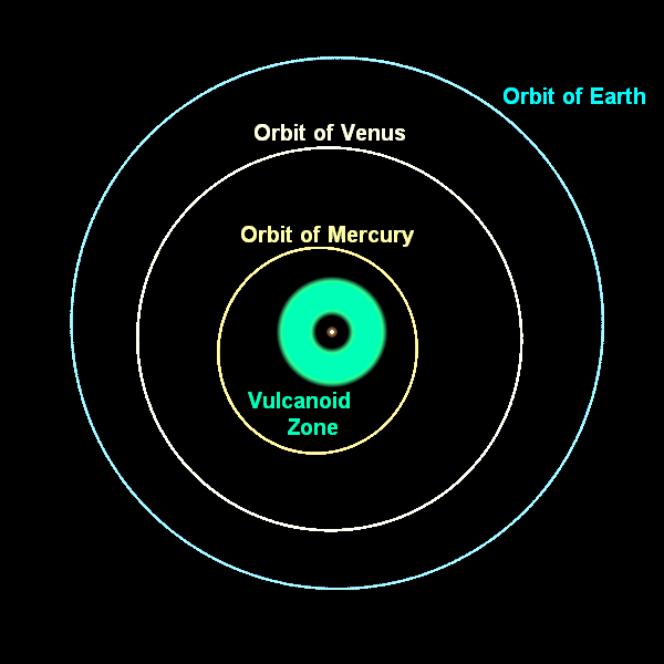 But “Vulcan, Mercury, Venus, Earth, Mars, Jupiter, Saturn, Uranus, Neptune, Pluto” is probably not the list of planets you learned in elementary school! Unlike the success with Neptune, Newtonian gravity was not going to be vindicated by discovery of another predicted planet. Rather than an unaccounted-for planet, the anomalous precession of Mercury, we now know, as Einstein figured out in September of 1915, is due to a failure of Newton’s theory of gravity. At slow speeds and for weak gravitational fields the Newtonian theory is an excellent approximation to Einstein’s theory -- so the largest errors in the Newtonian theory show up for the fastest-moving planet orbiting closest to the Sun.
Amazingly, thinking about a theory that explains experiments with electricity and magnets, and trying to reconcile it with Newton’s laws of gravitation and motion, had led to a solution to this decades-old problem in solar system dynamics. The theory has gone on from success to success since that time, most recently with the detection of gravitational waves first reported in 2016. It is of practical importance in the daily lives of many of us: GPS software written based on Newtonian theory rather than Einstein’s theory would be completely useless.
The Expansion of Space
More important to our subject, Einstein’s theory allowed for better-informed speculation about the history of the universe as a whole. In the years following Einstein’s November 1915 series of lectures, a number of theoreticians calculated solutions of the Einstein equations for highly-idealized models of the universe. The Einstein field equations are extremely difficult to solve in generality. The first attempts at solving these equations for the universe as a whole thus involved extreme idealization. They used what you might call “the most spherical cow approximation of all time.” They approximated the whole universe as completely homogeneous; i.e., absolutely the same everywhere.
We now know that on very large scales, this is a good approximation to our actual universe. To illustrate what we mean by homogeneity being a good approximation on very large scales, we have the figure below which shows a slice from a large-volume simulation of the large-scale structure of our universe. In these images, brighter regions are denser regions. The image has two sets of sub-boxes: large ones and small ones. We can see that the universe appears different in the small boxes. Box 4 is under dense, Box 5 is over dense, and Box 6 is about average. If we look at the larger boxes, the universe appears more homogeneous. Each box looks about the same. This is the sense by which we mean that on large scales the universe is highly homogeneous.

On large scales the Universe is highly homogeneous. The large boxes (boxes 1, 2, and 3) are about 200 Mpc across (that's about 600 million light years). No matter where you put down such a large box, the contents look similar. For the smaller boxes this is not the case. Images are from the Millenium Simulation.
Gif of an expanding grid (below) Image by Alex Eisner
D vs. z: Low z
In 1929, Edwin Hubble made an important observation by measuring distances to various galaxies and by measuring their "redshifts." Hubble inferred distances to galaxies by using standard candles, which are objects with predictable luminosities. Since farther away objects appear dimmer, one can predict distances by comparing the object’s expected luminosity with how bright it appears. The redshift of a galaxy, which cosmologists label as “z”, tells us how the wavelength of light has shifted during its propagation. Mathematically, 1+z is equal to the ratio of the wavelength of observed light to the wavelength of emitted light: (1+z=λobserved/λemitted). At least for z<<1, one can think of this as telling us how fast the galaxy is moving away from us according to the Doppler effect: a higher redshift indicates a larger velocity with relationship v=cz with c the speed of light. If a galaxy were instead moving towards us, its light would appear blueshifted. Hubble found that not only were nearly all the galaxies redshifted, but there was a linear relationship between the galaxies’ distances and redshifts. This is represented by Hubble’s law, v=H0d. Hubble's observations, which were evidence for this simple law, had profound consequences for our understanding of the cosmos: they indicated that the universe was expanding.
To understand this, take a look at the image of an expanding grid. Each of the two red points is “stationary”; i.e., they each have a specific defined location on the grid and do not move from that location. However, as the grid itself expands, the distance between the two points grows, and they appear to move away from each other. If you lived anywhere on this expanding grid, you would see all other points moving away from you. It's easiest to see this is true for the central location on the grid. Try placing your mouse over different points on the grid and following them as they expand. You will notice that points farther from the center will move away faster than points close to the center. This is how Hubble’s law and the expansion of space works. Instead of viewing redshifts as being caused by a Doppler effect from galaxies moving through space, we will come to understand the redshift as the result of the ongoing creation of new space.
Hubble’s constant, H0, tells us how fast the universe is expanding in the current epoch. It was first estimated to be about 500 km/s/Mpc, but after eliminating some gross systematic errors and obtaining more accurate measurements, we know this initial estimate was off, and not by any small amount. It's wrong by about a factor of 7! The exact value of the Hubble constant is actually somewhat controversial today, but everyone agrees it's somewhere between 66 and 75 km/s/Mpc. This means that on large length scales, where the approximation of a homogeneous universe becomes more accurate, about 70 kilometers of new space are created each second in every Megaparsec.
D vs. z: High z
As we will see, from Einstein’s theory of space and time we can expect the rate of expansion of space to change over time. The history of these changes to the expansion rate leave their impact on the distance-redshift relation if we trace it out to sufficiently large distances and redshifts. As we measure out to larger distances, the relationship is no longer governed by cz = H0 d. Instead, we will show that the redshift tells us how much the universe has expanded since light left the object we are observing.
1+z=λobservedλemitted=a0ae
where a is the “scale factor” that parameterizes the expansion of space, a0 is the scale factor today and ae is the scale factor when the light was emitted. We can observe quasars so far away that the universe has expanded by a factor of 7 since the light left them that we are receiving now. For such a quasar we have a0/ae = 7 so the wavelength of light has been stretched by a factor of 7, and by definition of redshift z we have z = 6.
The distance from us to such a quasar depends on how long it took for the universe to expand by a factor of 7. If the expansion rate were slower over this time, then it would have taken longer, so the quasar must be further away. Measurements of distance vs. redshift are thus sensitive to the history of the expansion rate.
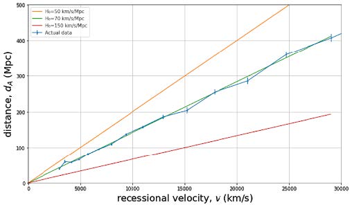
As we will see, how the expansion rate changes over time depends on what the universe is made out of. Therefore, studying D vs. z out to high distances and redshifts can help us determine the composition of the universe. We can see such measurements in Fig. B, together with some model curves. The models all have the same expansion rate today, H0, but differ in the mix of different kinds of matter/energy in the universe. A model that’s purely non-relativistic matter, the green dashed line "CDM Model", does a very poor job of fitting the data. The data seem to require a contribution to the energy density that we call “vacuum energy” or “the cosmological constant.” The “Lambda CDM” or "LCDM" model has a mixture of this cosmological constant and non-relativistic matter. The cosmological constant causes the expansion rate to accelerate. Thus, compared to the model without a cosmological constant (the "CDM Model"), the expansion rate in the past was slower; it thus took a longer time for the universe to expand by a factor of 1+z, and thus objects with a given z are at further distances. This acceleration of the expansion rate, discovered via D vs. z measurements at the end of the 20th century, was a great surprise to most cosmologists. Why there is a cosmological constant, or whether there is something else causing the acceleration, is one of the great mysteries of modern cosmology.

Overview Part II: The Hot Big Bang and its Relics
The expansion of the universe implies that it must have been much smaller, and much denser, in the past. If this is true, we should be able to see some consequences from the very high density period of the early universe. One such consequence is the relative abundances of light elements we see today. Most of the Helium, the second-most-common element in the Universe, was created when the expansion was less than a few minutes old. Trace amounts of other light elements were also created in this early period in a process we call Big Bang Nucleosynthesis (BBN). Observation of the abundances of these light elements can tell us about conditions at such early times. To achieve consistency between predictions and observations requires that the big bang was very hot, and thereby led to the prediction of what we call the cosmic microwave background. The discovery of this background in 1964 led to the establishment of the hot big bang model as the standard cosmological paradigm.
Our First Relic: Light Elements
In 1948, Gamow explored the very early universe as a source of elements heavier than hydrogen. He extrapolated Einstein’s theory of an expanding universe with certain assumptions about the composition of the universe and concluded that it was infinitely dense at a finite time in the past. He theorized that this early universe could be a prodigious source of heavier elements. If the universe began at infinitely high density and temperatures and underwent rapid expansion and cooling, atomic nuclei would form not too early, when high-energy radiation did not permit any nuclei to survive, and not too late, when temperatures were too low for the nuclear collisions to overcome the Coulomb repulsion, but at a just-right intermediate stage.
As we will see, almost all of the hydrogen and helium in the universe originated in the big bang. Further, those are the only elements to be produced in the big bang in anything beyond trace amounts. In our chapters on big bang nucleosnythesis we will explore the theory of the production of helium, and compare the predicted amounts of helium and trace amounts of deuterium and lithium with attempts to infer those abundances from observations.
Our Next Relic: The Cosmic Microwave Background
An important aspect of Gamow's work was that in order to avoid overproduction of helium and other heavy elements, the ratio of nucleons to photons at this just-right epoch had to be very small. Since the number of photons in black body radiation is proportional to temperature cubed, this means that the “Big Bang” had to be very, very hot. Pushing this chain of logic forward in a follow-up paper, Alpher and Herman theorized that we should see a background of heat and light from this period of high temperature and photon density. This background was discovered later in 1964 and is known as the Cosmic Microwave Background (CMB).
The CMB is an enormous gift from nature to cosmologists. By measuring both the spectrum of this light, and mapping its variation in intensity and polarization across the sky, we have a highly sensitive probe of conditions in the universe from times of thousands of years to hundreds of thousands of years. What's more, the conditions in the universe at this time were such that one can calculate, with great accuracy, the outcomes for the CMB spectrum, intensity, and polarization measurements, to be expected for some particular model of the cosmos. Physical systems with such extreme calculability and utility are rare. The CMB is to cosmology what the solar system was for science and Newtonian gravitational theory three hundred plus years ago.
The following image is a projection of intensity variations across the whole (curved) sky on to a flat map. To better understand how this relates to what we observe from Earth, explore the virtual CMB planetarium below it by clicking and dragging. This shows how the CMB would look over a tree-lined horizon, if human eyes were extremely sensitive to light at millimeter wavelengths.

CMB Planetarium
As we will see, the consistency between the statistical properties of CMB anisotropy and polarization maps, and the predictions of the standard cosmological model, LCDM, are quite extraordinary. They give us some confidence that we know what we are talking about when we describe conditions in the universe when it is just a few hundred thousand years old and even younger.
Other Relics of the Big Bang: the Cosmic Neutrino Background and Dark Matter
The hot and dense conditions of the big bang not only led to thermal production of a background of photons (the CMB), but also a background of neutrinos, and possibly dark matter as well. According to our standard cosmological model, most of the mass/energy density of the universe was at one time (just prior to the epoch of Big Bang Nucleosythesis) in the Cosmic Neutrino Background (CNB). This background has yet to be directly detected, but has been detected via its gravitational influence on the photons.
To explain a long list of different observed phenomena, our standard cosmological model also includes a significant amount of non-relativistic matter that does not interact with atoms, nuclei, and light, that we call "dark matter." The amount of dark matter in a large representative sample of the universe appears to be about six times the density of matter made of out of atomic nuclei and electrons. To date we only know of this dark matter via its gravitational influence; it has not yet been directly detected. Dark matter might also be a thermal relic of the Big Bang.
Conclusion
The agreement between cosmological predictions and observations give us a high degree of confidence that our models are capturing some important and true things about the nature of the cosmos. However, we still don’t know what most of the universe is made of, or how it came into existence. There is work left to do!
Our measurements are constantly improving, and one never knows when a combination of precise measurements and predictions will reveal something new and interesting about the universe, or when a theoretical insight will resolve some long-standing puzzles and shine a light for us to follow towards a more perfect understanding.
The adventure continues. Maybe you will join us in our quest!