
1.37: Redshifts


- Last updated
- Jan 5, 2023
- Save as PDF

( \newcommand{\kernel}{\mathrm{null}\,}\)
We introduced expanding, non-Euclidean spacetimes in the previous chapter. Now we begin to work out observational consequences of living in such a spacetime. In this and the next two chapters we will derive Hubble's Law, v=H0d. In fact, we will derive a more general version of it valid for arbitrarily large distances.
In Minkowski space, the invariant distance, ds, between spacetime point (t,x,y,z) and another one at (t+dt,x+dx,y+dy,z+dz) is given by:
ds2=−c2dt2+dx2+dy2+dz2
We call it invariant because it is invariant under Lorentz transformations. Physically, for ds2>0, ds is the length of a ruler with one end on each of the two space-time points, if the ruler is at rest in a frame in which the two space-time points are simultaneous. For ds2<0, √−ds2/c is the amount of time that elapses on a clock that passes from one space-time point to the other.
In spherical coordinates the above expression for the invariant distance becomes:
ds2=−c2dt2+dr2+r2(dθ2+sin2θdϕ2)
More generally, the invariant distance in a spatially homogeneous and isotropic Universe can be written as:
ds2=−c2dt2+a2(t)[dr21−kr2+r2(dθ2+sin2θdϕ2)]
Such spacetimes are known as Friedmann-Robertson-Walker (FRW) models, or sometimes just Robertson-Walker, and sometimes Friedmann-Robertson-Walker-Lemaitre models.
We are now ready to define "redshift" and derive the relationship between it and the expansion of space. Redshift is a quantification of the stretching of the wavelength of light. We use the symbol z to denote redshift and define it as:
z≡(λreceived−λemitted)/λemitted.
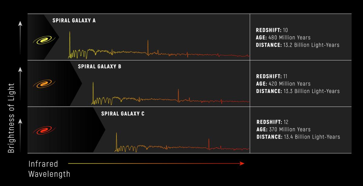
We see in the figure below (from NASA and Space Telescope Science Institute) some model spectra of galaxies with redshifts of 10, 11, and 12. One can see in the image that the same spectral features appear at longer wavelengths as the redshift increases. These features all had the same wavelength when emitted, but those wavelengths get stretched by the expansion to longer wavelengths. The further away the objects, the greater the stretching that occurs. We will explore this relationship between distance and redshift in chapter 8.
Next we will derive the relationship between redshift and expansion for light that leaves an object at rest at time te and is observed today by an observer at rest at time tr. We'll get there with the following two exercises.
Note
By "at rest" we mean at rest in the coordinate system that has an invariant distance of the form in Equation ???. This frame is called "cosmic rest." Note that for a frame that is moving with respect to cosmic rest, slices of constant time would be different, and we'd no longer have this simple form where the scale factor only depends on the time coordinate.
Box 1.37.1
Exercise 6.1.1: Show that if Δte is the time interval between emitted light pulses (as measured by a stationary observer located where the emission is happening) and if Δtr is the time interval between reception of first pulse and second pulse (as measured by a stationary observer located where the reception is occurring) then Δtr/Δte=a(tr)/a(te). To do so, use conformal time defined by dτ=dt/a(t) and draw the pulse trajectories on an x vs. τ diagram. By stationary observer we mean one that is at a constant value of x; i.e., is at rest in the cosmic rest frame. You can assume that Δtr and Δte are very short time scales compared to the time scale over which a(t) changes appreciably. Practical applications of this result often have a(t) changing on billion-year time scales and the Δts shorter than nanoseconds so this assumption is well justified!
- Answer
-

It's clear from the graphic that Δτe=Δτr. We can integrate up dτ=dt/a(t) by approximating a(t) as constant over these short time intervals to get Δτ=Δt/a(t). Then we can easily see that Δtr/Δte=a(tr)/a(te).
Box 1.37.2
Exercise 6.2.1: Imagine propagation of electromagnetic waves. Use the above result to show that the wavelength of the waves emitted at time tr and observed at time te is stretched so that:
z≡(λreceived−λemitted)/λemitted=a(tr)/a(te)−1
Hint: think about what happens to the period of the wave first, and then go from that to wavelength using the fact that wavelength is proportional to period.
Box 1.37.3
Exercise 6.3.1: The most distant object for which a redshift has been measured is called a gamma-ray burst and it has a redshift of z=8.2. By what factor has the universe expanded since light left that object?
We have just worked out the amazing fact that if we can identify a spectral line and measure its wavelength, then we can directly determine how much the universe has expanded since light left the object. Rearranging the result from Exercise 6.2.1 a little we can express this amazing fact as an equation:
1+z=λr/λe=a(tr)/a(te).
Look again at the figure above and notice that the more distant the object, the higher the redshift. This is because the more distant the object, the more time it took light to get to us from the object, and therefore the smaller the scale factor was at the time the light left the object, te.
Before closing this section, we remind the reader of how redshifts due to the Dopper effect are related to speed -- a result we will use later in deriving Hubble's Law. If a source is moving away from you at speed v and emitting pulses with period T, then the second pulse has to travel a distance vT further to get to you than was the case for the first pulse. So it's arrival will be delayed by a time vT/c. Thus the period for the arriving pulses is T(1+v/c). Since wavelength is proportional to period this means the wavelength is stretched by a factor of 1+v/c, which means, by definition of the redshift z, that z=v/c. Note that our derivation has ignored the effect of relativistic time dilation. If the source had period T at rest, then if it were moving with speed v with respect to us, in our frame the period would be stretched to γT and so the complete expression for z from the Doppler effect is 1+z=γ(1+v/c). But we are only interested in this expression for small v/c, for which γ∼1.
Summary
- In an expanding homogeneous and isotropic universe, the ratio between the wavelength of light emitted by an observer at cosmic rest, λe at time te and the wavelength as measured by an observer at cosmic rest λr at time tr is given by 1+z≡λr/λe=a(tr)/a(te) where a(t) is the scale factor at time t and the above equation defines the redshift z. We can think of this as the wavelength stretching with the expansion.
- In a non-expanding universe, a source moving away from an observer with v/c≪1 has its light redshifted (wavelength stretched) by λr/λe=1+v/c which is the normal Doppler effect you have studied before. What this implies is that if we interpret a small redshift z caused by the expansion of space as due to an ordinary motion-induced Dopper effect we will set z=v/c. We will use this relationship later in our derivation of Hubble's Law: v=H0d.
Additional Resources
You can look at images and spectra of galaxies in the Sloan Digital Sky Survey here. The spectra include identification of emission and absorption lines (with the atoms or ions responsible for them) and measurements of the redshift. To find the spectra and images, look for the table and click on the Object ID.
Quasar absorption line systems have particularly interesting spectra. You can read about them here.