
1.26: The Spectrum of the CMB
- Page ID
- 55895

\( \newcommand{\vecs}[1]{\overset { \scriptstyle \rightharpoonup} {\mathbf{#1}} } \)
\( \newcommand{\vecd}[1]{\overset{-\!-\!\rightharpoonup}{\vphantom{a}\smash {#1}}} \)
\( \newcommand{\dsum}{\displaystyle\sum\limits} \)
\( \newcommand{\dint}{\displaystyle\int\limits} \)
\( \newcommand{\dlim}{\displaystyle\lim\limits} \)
\( \newcommand{\id}{\mathrm{id}}\) \( \newcommand{\Span}{\mathrm{span}}\)
( \newcommand{\kernel}{\mathrm{null}\,}\) \( \newcommand{\range}{\mathrm{range}\,}\)
\( \newcommand{\RealPart}{\mathrm{Re}}\) \( \newcommand{\ImaginaryPart}{\mathrm{Im}}\)
\( \newcommand{\Argument}{\mathrm{Arg}}\) \( \newcommand{\norm}[1]{\| #1 \|}\)
\( \newcommand{\inner}[2]{\langle #1, #2 \rangle}\)
\( \newcommand{\Span}{\mathrm{span}}\)
\( \newcommand{\id}{\mathrm{id}}\)
\( \newcommand{\Span}{\mathrm{span}}\)
\( \newcommand{\kernel}{\mathrm{null}\,}\)
\( \newcommand{\range}{\mathrm{range}\,}\)
\( \newcommand{\RealPart}{\mathrm{Re}}\)
\( \newcommand{\ImaginaryPart}{\mathrm{Im}}\)
\( \newcommand{\Argument}{\mathrm{Arg}}\)
\( \newcommand{\norm}[1]{\| #1 \|}\)
\( \newcommand{\inner}[2]{\langle #1, #2 \rangle}\)
\( \newcommand{\Span}{\mathrm{span}}\) \( \newcommand{\AA}{\unicode[.8,0]{x212B}}\)
\( \newcommand{\vectorA}[1]{\vec{#1}} % arrow\)
\( \newcommand{\vectorAt}[1]{\vec{\text{#1}}} % arrow\)
\( \newcommand{\vectorB}[1]{\overset { \scriptstyle \rightharpoonup} {\mathbf{#1}} } \)
\( \newcommand{\vectorC}[1]{\textbf{#1}} \)
\( \newcommand{\vectorD}[1]{\overrightarrow{#1}} \)
\( \newcommand{\vectorDt}[1]{\overrightarrow{\text{#1}}} \)
\( \newcommand{\vectE}[1]{\overset{-\!-\!\rightharpoonup}{\vphantom{a}\smash{\mathbf {#1}}}} \)
\( \newcommand{\vecs}[1]{\overset { \scriptstyle \rightharpoonup} {\mathbf{#1}} } \)
\(\newcommand{\longvect}{\overrightarrow}\)
\( \newcommand{\vecd}[1]{\overset{-\!-\!\rightharpoonup}{\vphantom{a}\smash {#1}}} \)
\(\newcommand{\avec}{\mathbf a}\) \(\newcommand{\bvec}{\mathbf b}\) \(\newcommand{\cvec}{\mathbf c}\) \(\newcommand{\dvec}{\mathbf d}\) \(\newcommand{\dtil}{\widetilde{\mathbf d}}\) \(\newcommand{\evec}{\mathbf e}\) \(\newcommand{\fvec}{\mathbf f}\) \(\newcommand{\nvec}{\mathbf n}\) \(\newcommand{\pvec}{\mathbf p}\) \(\newcommand{\qvec}{\mathbf q}\) \(\newcommand{\svec}{\mathbf s}\) \(\newcommand{\tvec}{\mathbf t}\) \(\newcommand{\uvec}{\mathbf u}\) \(\newcommand{\vvec}{\mathbf v}\) \(\newcommand{\wvec}{\mathbf w}\) \(\newcommand{\xvec}{\mathbf x}\) \(\newcommand{\yvec}{\mathbf y}\) \(\newcommand{\zvec}{\mathbf z}\) \(\newcommand{\rvec}{\mathbf r}\) \(\newcommand{\mvec}{\mathbf m}\) \(\newcommand{\zerovec}{\mathbf 0}\) \(\newcommand{\onevec}{\mathbf 1}\) \(\newcommand{\real}{\mathbb R}\) \(\newcommand{\twovec}[2]{\left[\begin{array}{r}#1 \\ #2 \end{array}\right]}\) \(\newcommand{\ctwovec}[2]{\left[\begin{array}{c}#1 \\ #2 \end{array}\right]}\) \(\newcommand{\threevec}[3]{\left[\begin{array}{r}#1 \\ #2 \\ #3 \end{array}\right]}\) \(\newcommand{\cthreevec}[3]{\left[\begin{array}{c}#1 \\ #2 \\ #3 \end{array}\right]}\) \(\newcommand{\fourvec}[4]{\left[\begin{array}{r}#1 \\ #2 \\ #3 \\ #4 \end{array}\right]}\) \(\newcommand{\cfourvec}[4]{\left[\begin{array}{c}#1 \\ #2 \\ #3 \\ #4 \end{array}\right]}\) \(\newcommand{\fivevec}[5]{\left[\begin{array}{r}#1 \\ #2 \\ #3 \\ #4 \\ #5 \\ \end{array}\right]}\) \(\newcommand{\cfivevec}[5]{\left[\begin{array}{c}#1 \\ #2 \\ #3 \\ #4 \\ #5 \\ \end{array}\right]}\) \(\newcommand{\mattwo}[4]{\left[\begin{array}{rr}#1 \amp #2 \\ #3 \amp #4 \\ \end{array}\right]}\) \(\newcommand{\laspan}[1]{\text{Span}\{#1\}}\) \(\newcommand{\bcal}{\cal B}\) \(\newcommand{\ccal}{\cal C}\) \(\newcommand{\scal}{\cal S}\) \(\newcommand{\wcal}{\cal W}\) \(\newcommand{\ecal}{\cal E}\) \(\newcommand{\coords}[2]{\left\{#1\right\}_{#2}}\) \(\newcommand{\gray}[1]{\color{gray}{#1}}\) \(\newcommand{\lgray}[1]{\color{lightgray}{#1}}\) \(\newcommand{\rank}{\operatorname{rank}}\) \(\newcommand{\row}{\text{Row}}\) \(\newcommand{\col}{\text{Col}}\) \(\renewcommand{\row}{\text{Row}}\) \(\newcommand{\nul}{\text{Nul}}\) \(\newcommand{\var}{\text{Var}}\) \(\newcommand{\corr}{\text{corr}}\) \(\newcommand{\len}[1]{\left|#1\right|}\) \(\newcommand{\bbar}{\overline{\bvec}}\) \(\newcommand{\bhat}{\widehat{\bvec}}\) \(\newcommand{\bperp}{\bvec^\perp}\) \(\newcommand{\xhat}{\widehat{\xvec}}\) \(\newcommand{\vhat}{\widehat{\vvec}}\) \(\newcommand{\uhat}{\widehat{\uvec}}\) \(\newcommand{\what}{\widehat{\wvec}}\) \(\newcommand{\Sighat}{\widehat{\Sigma}}\) \(\newcommand{\lt}{<}\) \(\newcommand{\gt}{>}\) \(\newcommand{\amp}{&}\) \(\definecolor{fillinmathshade}{gray}{0.9}\)No other natural source of radiation has ever been measured to be as consistent with black-body radiation as is the case with the CMB. Here we look at the measurements of the spectrum from a Nobel-prize winning instrument on the COBE satellite, before turning to the question of why the CMB is so near to being a black body and what we can learn from that. We will see that this is expected based on a very early epoch in which a thermal distribution is established by kinetic-energy-changing, and photon-number-changing interactions, and subsequent epochs in which passive evolution under the expansion of space preserves the thermal distribution achieved earlier, albeit with a temperature that decreases as the universe expands. The very high number of photons relative to matter also plays a role in making the CMB a better approximation of a black body than is the case for the Sun, for example.
The Spectrum Observed
NASA's COsmic Background Explorer (COBE) satellite was launched in 1989 with three scientific instruments on board, two of which would lead to Nobel prize-worthy discoveries. One of these two was the Far Infrared Absolute Spectrometer, or FIRAS. The precision and accuracy of the FIRAS measurements were extraordinary. The figure below shows the spectrum of the CMB as determined from FIRAS data. The measurements are so precise that the width of the error bars is smaller than the thickness of the theoretical black body spectrum curve. You can read the original paper describing the FIRAS measurements and determination of this spectrum here: https://iopscience.iop.org/article/10.1086/178173/pdf.
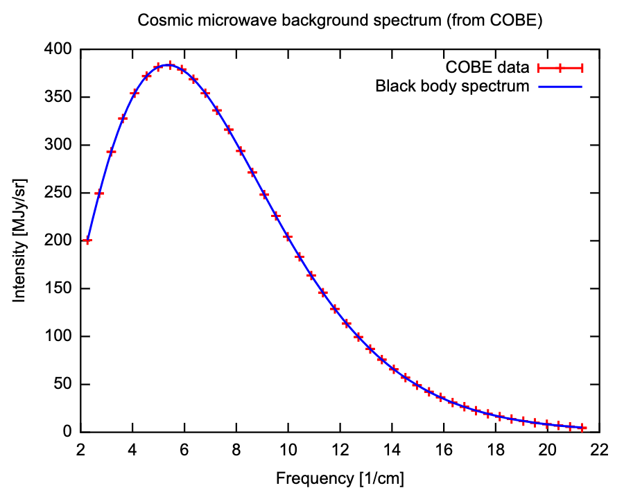
The "Intensity" plotted on the y axis is telling us the energy per unit amount of sky (solid angle) per unit interval of frequency flowing through a unit area per unit time. The units are MJy/sr where "Jy" stands for Jansky with 1 Jansky = \(10^{-23} \) erg/s/cm\(^2\)/Hz and "sr" is short for steradian, a unit of solid angle. The \(x\) axis is the frequency in units of 1/cm -- which is an unusual way of expressing frequency. To convert to more familiar units, one multiplies by the speed of light, which is about \(3 \times 10^{10}\) cm/sec so, for example, 10 cm\(^{-1}\) is about 300 GHz.
Theoretical Prediction
According to our standard thermal history, reactions that create and destroy photons were fast enough at \(z \ge 10^7\) to drive the CMB photons into a black body distribution; i.e., a thermal distribution with zero chemical potential (for massless bosons). In terms of the phase space distribution function, \(f\) we have
\[f = \frac{1}{\exp(pc/k_BT) -1}. \]
So that's true for \(z \ge 10^7\). What about today? We need to work that out in order to compare with observations we can do today. At \(z \le 10^7\) the number changing reactions are slow so we are not guaranteed that the photon chemical potential remains zero. Let's work out what happens under the assumption that no new energy is injected into the photon distribution (by an unstable particle that has decay byproducts that include photons, for example). Let's do so by tracking what happens to photons in a small region of momentum space initially centered on momentum \(\vec p_i\) with volume \(V_{p,i}\), and in some comoving volume, with initial physical volume \(V_{x,i}\). We've taken the phase space volume to be small enough that \(f\) does not vary by much across it. So we don't need to integrate to find the total number of particles, we can just multiply:
\[N_i = f(p_i;T_i) V_{x,i} V_{p,i}.\]
Let's, for now, ignore scattering interactions that the photons have and treat them as if they are not receiving any kinetic energy from scattering. In this case their momenta are just redshifting with the expansion so that at some later point in evolution, when the scale factor has gone from \(a_i\) to \( a_f\), we have \(p_f = p_i a_i/a_f\). Also due to the redshifting of momentum, the momentum-space volume that contains these photons shrinks by a factor of \((a_i/a_f)^3\), and the physical volume of the comoving volume we are tracking grows by \((a_f/a_i)^3\). So we have
\[ \begin{align} N_f &= f(p_f;T_i) V_{x,f}V_{p,f} \\[4pt] &= f(p_f;T_i) \left(\dfrac{a_f}{a_i}\right)^3V_{x,i}\left(\dfrac{a_i}{a_f}\right)^3V_{p,i} \\[4pt] &= f(p_f;T_i) V_{x,i}V_{p,i}. \end{align}\]
Box \(\PageIndex{1}\)
Exercise 28.1.1: Draw the Cartesian axes of a 2-dimensional momentum space (\(p_x,p_y\)) and also of a 2-dimensional configuration space (\(x,y\)). Draw a box centered on the origin of the configuration space and one around some region of the momentum space, representing boxes bounding the particles we are going to track from one time to another. Take this first drawing as for the initial time, and make a subsequent pair of graphs for the later time, with the sizes and locations of these boxes evolving appropriately, following the above discussion. Take the configuration space coordinates to represent physical distances of particles from the origin; i.e., these are not comoving coordinates.
How is \(N_f\) related to \(N_i\)? By design we've tried to keep these two equal. We've shifted the region of momentum space to track the photons as they redshift. So none of them have moved out of our momentum-space region due to how the momentum has changed. They are moving through space in different directions, so some will leave our comoving spatial volume. But, due to homogeneity and isotropy, the same number will flow in as flow out. The net result is that \(N_f = N_i\). From this we can conclude that
\[\begin{align} f(p_f;T_i, t_f) = f(p_i;T_i,t_i) &=\frac{1}{\exp(p_ic/k_BT_i)-1} \\[4pt] &= \frac{1}{\exp(p_f (a_f/a_i)c/k_BT_i)-1 }= \frac{1}{\exp(p_f c/(k_BT_i a_i/a_f))-1} \\[4pt] &= \frac{1}{\exp(p_fc/k_BT_f)-1} \end{align}\]
with \(T_f = T_i \dfrac{a_i}{a_f}\).
This is a remarkable result. Even though we ignored all interactions, the things that maintain equilibrium, we find out that such evolution results in a phase space distribution function that is the same as one would get for thermal equilibrium with zero chemical potential, although at a reduced temperature. The expansion of the universe cools the gas of photons while maintaining a chemical-potential-free thermal distribution.
We have ignored any energy that might be imparted to the photons by the electrons. But any such energy is very small since, in a given region of space, the total kinetic energy in the electrons is much less than the total kinetic energy in the photons, mainly because of how the photons greatly outnumber the electrons. The bottom line is that we expect, to a good approximation, the photons today to have a phase space distribution function for massless bosons in thermal equilibrium with zero chemical potential. Given that they have two degrees of freedom, this is a Planck distribution.