
1.30: Structure Formation


( \newcommand{\kernel}{\mathrm{null}\,}\)
Shortly before the epoch of the CMB, matter became the dominant constituent of the universe. Throughout the matter-dominated epoch---i.e., from a few hundred thousand years after the Big Bang until dark energy--matter equality nearly 13 billion years later---dark matter and baryonic structure formed and grew. This Chapter describes how, under the gravitational influence of dark matter, small fluctuations in the matter density field evolve. Particularly dense regions collapse into nonlinear, self-gravitating systems called dark matter halos, which form the nodes of the cosmic that cosmologists observe today.
Linear Structure Formation
A key quantity used to describe dark matter structure is the density field ρ(→r,a), which specifies the matter density ρ (i.e., the mass contained in some volume V) as a function of three-dimensional position →r and scale factor a. Specifically, consider the density contrast
δ(→r,a)=ρ(→r,a)−ˉρ(a)ˉρ(a),
where ˉρ(a) is the mean matter density at a given epoch. The density contrast describes how matter is distributed relative to the mean density; at a given location and time, δ>0 (δ<0) corresponds to an overdense (underdense) region, and δ=0 corresponds to a region of average density. We refer to structure on a given scale as linear when |δ|≪1 and nonlinear when |δ|≈1. Linear structure formation can largely be modeled analytically, while nonlinear structure formation requires numerical simulations to model accurately.
How does δ evolve over time, and what are its typical values at early times and today? Recall the Friedmann equation from Chapter 11:
H2=(˙aa)2=8πGˉρ3,
where we assume that the universe is flat (k=0) and use ˉρ to denote the density is averaged over a large region of the universe. Technically, the density that enters the Friedmann equation is the sum of matter, radiation, and dark energy, but this sum is dominated by matter during the matter-dominated epoch.
Consider a region of the universe with some local matter density ρ. That region will either be overdense and behave locally like a closed universe, or underdense and behave locally like an open universe. Thus, this region obeys
H2=(˙aa)2=8πGρ3−ka2
⟹ρ−ˉρ∝ka2
⟹δ=ρ−ˉρˉρ∝1ˉρa2∝a3a2∝a,
where Equation ??? follows by subtracting Equations ??? and ???, and the final line uses ˉρ∝a−3 as appropriate for non-relativistic matter. For a more rigorous derivation of this scaling, see Problem 31.1.
As the universe expands, overdense regions with δ>0 become denser relative to the background according to Equation ???. Gravity attracts matter surrounding a given overdensity towards its center, slowing down the expansion of overdense regions relative to the background and causing their density contrast to grow.
Box 1.30.1
Exercise 31.1.1: Qualitatively describe how underdense regions evolve in the linear regime. Does their density contrast increase or decrease as the universe expands? Justify your answer mathematically.
At the time of the CMB, baryon density fluctuations have an average size of
δbaryon(aCMB)∼Δρbaryonˉρbaryon∼ΔTbaryonˉTbaryon≈10−5.
According to Equation ???, the average size of these fluctuations today is therefore
δbaryon(atoday)≈atodayaCMBδbaryon(aCMB)≈103δbaryon(aCMB)≈10−2.
This is not what we observe! Instead, today's universe is filled with galaxies, which have densities larger than the background by orders of magnitude. In other words, large, non-baryonic density fluctuations must be present at the time of the CMB in order for nonlinear structure to form by today. These density fluctuations are sourced by dark matter. Problem 31.2 explores why baryonic perturbations are much smaller than dark matter perturbations at the time of the CMB.
| Dark matter drives the growth of small baryonic overdensities observed in the CMB (left) into nonlinear structure traced by galaxies today (right). |
Nonlinear Structure Formation
What happens to overdensities as they near δ≈1? Consider a toy model in which a region of the universe has a uniformly higher matter density than the rest,
ρ(r,ti)=ˉρ(ti){1+δi,r<Ri1,r>Ri
where r is the radial distance from the center of the overdensity, Ri is the initial size of the overdensity, ti is the initial time, ˉρ(ti) is the background density, and δi is the size of the overdensity. This is referred to as a top-hat overdensity.
Problem 31.3 explores the evolution of this system. The overdensity initially expands with the Hubble flow; if δi>Ωm(ti)−1−1, gravitational attraction overwhelms the expansion, and the region collapses. This picture schematically describes how self-gravitating dark matter halos form.
Box 1.30.2
Exercise 31.2.1: Realistic cosmological density fluctuations are more complex than the top-hat model for several reasons:
- Overdensities are not spatially uniform; instead, the density contrast is higher near the centers of overdensities and decreases until joining onto the mean density;
- Fluctuations are not spherically symmetric; instead, collapse occurs successively along the major, intermediate, and minor axes of the initial perturbation;
- Collapse is not purely radial; particles orbiting an overdensity have angular momentum.
Qualitatively describe how each effect influences how overdensities evolve. Assuming that the overdensity will collapse, do you expect each effect to speed up or slow down the process?
Gravitational collapse naturally leads to bottom-up (or hierarchical) structure formation. Consider a shell of matter at distance r from the center of an overdensity as it collapses after turnaround. The time taken for this shell to collapse is given by
tff∼√r/g∼√r3/(GM)∼√1/(Gρ),
where M is the enclosed mass and ρ is the enclosed density. This timescale, referred to as the free-fall time, is relevant in many other astrophysical settings where gravity plays an important role.
Matter fluctuations have higher average densities at early times because the background matter density is higher (even though overdensities are smaller at early times). Thus, according to Equation ???, small overdensities at early times collapse more quickly than large overdensities at later times. These small overdensities collapse, forming small dark matter halos, which merge together to form ever larger structures. The typical masses of these first-generation halos depend on the properties of dark matter and the primordial power spectrum. They are typically at least 10 orders of magnitude smaller than the most massive (≈1015 M⊙) clusters today; in many models, including weakly interacting massive particle (WIMP) dark matter, the first halos are even smaller (≈10−6 M⊙). In contrast, theories of neutrino dark matter considered in the 1970s predict top-down structure formation, in which "superclusters" form and subsequently fragment into smaller pieces. This scenario is ruled out by observations, which show that small galaxies and halos form first and subsequently merge to form massive objects.
Numerical simulations are used to predict the distribution and properties of halos over a wide range of mass scales and redshifts. In particular, cosmological N-body simulations solve for the gravitational evolution of discretized particles, which represent the dark matter density field, in an expanding FLRW universe. A key prediction of these simulations is the mass distribution of collapsed halos, or the halo mass function, which is predicted to increase as halo mass decreases in a roughly scale-invariant fashion:
dndM∝M−αhalo,
where n is the comoving number density of dark matter halos, M is halo mass, and α≈1.9.
Of course, it's difficult to compare predictions for the distribution of dark matter halos directly to observations. Chapter 32 explores how galaxies form in dark matter halos, and shows that the hierarchical structure formation paradigm describes observations of the nonlinear galaxy distribution today extremely well.
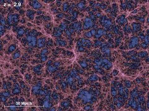 |
| Growth of dark matter structure in a cosmological N-body simulation. Pink (blue) regions correspond to overdensities (underdensities). Dark matter halos form, grow, and merge within the overdense regions, resulting in the cosmic web of structure cosmologists observe today. |
HOMEWORK Problems
Problem 1.30.1: The growth of linear dark matter overdensities.
This problem walks through a more rigorous derivation of the result δ∝a. The dynamics of the dark matter density field can be described using the following equations:
∂ρ∂t+∇⋅(ρ→v)=0
∂→v∂t+(→v⋅∇)→v=−∇pρ−∇Φ
∇2Φ=4πGρ,
where ρ is the dark matter density, →v is its velocity, p is its pressure, and Φ is the gravitational potential. Equations ??? (the continuity equation) enforces conservation of mass, Equation ??? (the Euler equation) enforces conservation of momentum, and Equation ??? (the Poisson equation) describes how matter sources the gravitational potential. Let
ρ(→r,t)=ˉρ(t)+Δρ(→r,t)=ˉρ(t)[1+δ(→r,t)]
→v(→r,t)=→v0(→r,t)+Δ→v(→r,t)
Φ(→r,t)=Φ0(→r,t)+ΔΦ(→r,t).
By plugging these into the fluid equations and keeping terms up to first order in the fluctuations δ, Δ→v, and ΔΦ, combining the equations yields a differential equation for the evolution of the density contrast:
¨ˆδ+2H˙ˆδ=(4πGˉρ−c2sk2a2)ˆδ,
where ˆδ is the Fourier transform of delta, k is the wavenumber associated with the Fourier transform, and c2s=∂p/∂ρ is the speed of sound. On large scales (small k), dark matter behaves as a pressureless fluid with cs=0. Thus,
¨ˆδ+2H˙ˆδ=32H2ˆδ.
a) Let ˆδ∝tn and solve for n by plugging this into Equation ???; you'll obtain two solutions for n because this is a second-order differential equation. Assume that the universe only contains matter to plug in H(t).
b) Interpret both solutions obtained in part a) physically. Show that one of the solutions yields the expected behavior δ∝a.
Problem 1.30.2: The growth of linear baryonic overdensities.
We argued that dark matter overdensities at the time of the CMB are large enough to facilitate nonlinear structure formation by today. But why are baryonic fluctuations smaller than dark matter fluctuations at early times? The key difference is that baryons can exchange energy and momentum by interacting with each other, and are therefore not a pressureless fluid. Thus, for baryons, we can't drop the c2s term in Equation ???.
The kinds of solutions to Equation ??? are determined by the sign of 4πGˉρ−c2sk2a2. At a given time, this depends on whether k is smaller or larger than a critical wavenumber kJ; the corresponding scale λJ=2π/kJ is referred to as the Jeans length.
a) Derive the Jeans length in terms of cs, a, and ˉρ.
b) Qualitatively describe how baryonic overdensities evolve on scales larger than and smaller than the Jeans length.
c) Before recombination, baryons feel pressure exerted by photons; the corresponding speed of sound is cs≈c/√3. Calculate the corresponding Jeans length assuming recombination occurs at z=1100. Relate this scale to the wavenumber of the peak in the linear matter power spectrum shown in the figure below (adapted from Chabanier et al. 2019).
Problem 1.30.3: Top-hat collapse.
Consider the top-hat perturbation defined in Equation ??? A shell at radius ri initially expands with the Hubble Flow, vi=H(ti)ri, and thus has an initial energy per unit mass (or specific energy) of
Ei=Ki+Ui=12v2i−GM(<ri)ri,
where M(<ri) is the enclosed mass. The integrated equation of motion for this shell is
12(drdt)2−GMr=E.
a) Show that the system collapses (corresponding to Ei<0) if δi>Ωm(ti)−1−1.
b) Show that r(θ)=A(1−cosθ), t(θ)=B(θ−sinθ) solves the integrated equation of motion, where θ∈[0,2π], A=GM/2|E|, and B=GM/(2|E|)3/2.
c) Run the code snippet and qualitatively describe the plotted evolution of the system. Is this qualitatively consistent with the description near Equation ????
Login with LibreOne to run this code cell interactively.
If you have already signed in, please refresh the page.
import numpy as np
import matplotlib.pyplot as plt
%matplotlib inline
%config InlineBackend.figure_format='retina'

###

#parametric solution in GM = 1 units
theta_array = np.linspace(1e-1,2*np.pi-1e-1,100)

def r_tophat(theta,E):
    A = 1./(2.*np.abs(E))
    return A*(1.-np.cos(theta))

def t_tophat(theta,E):
    B = 1./(2.*np.abs(E))**(1.5)
    return B*(theta-np.sin(theta))

###

#Plot evolution of system
plt.figure(figsize=(8,6))
E_array = np.linspace(-0.5,-0.1,5)

for E in E_array:
    plt.plot(t_tophat(theta_array,E),r_tophat(theta_array,E),label=r'$E=${:0.1f}'.format(E))

plt.xlabel(r'$t$',fontsize=16)
plt.ylabel(r'$r$',fontsize=16)
plt.legend(loc=1,fontsize=15)

plt.show()