A1: Spacetime Geometry

[The 'A' series of chapters is an alternative start to the textbook in which chapters 1 through 4 are skipped, so that we dive right into an expanding spacetime.] 

In this chapter we introduce the geometrical concept of a spacetime, how we describe it mathematically, and the relationship of the mathematical quantities to things we can measure with clocks and rulers. We begin with a spacetime we assume that you have studied before: the Minkowski spacetime of special relativity.  After some review of special relativity, to get everyone oriented to the notation, we then generalize the spacetime slightly to one that is uniformly expanding. With additional assumptions we then calculate the age of this spacetime as a function of expansion rate, as well as the "past horizon."

The Invariant Distance

We can label spacetimes with coordinates; for example, we could label every point in a spacetime with one spatial dimension (a so-called 1+1-dimensional spacetime) with a \(t\) value and an \(x\) value. These coordinates are just labels, with no physical meaning on their own. Physical meaning comes via a rule that connects infinitesimally-separated pairs of points to measurements with clocks and rulers. More specifically, the rule gives the square of the "invariant distance" between infinitesimally-separated pairs of points, which we denote as \(ds^2\). Before giving an example of such a rule, let's make completely precise the relationship between \(ds^2\) and what can be measured with clocks and rulers.

Note

The physical interpretation of \(ds^2\) is as follows:

1. For \(ds^2 < 0\) (which we call time-like separations), the time elapsed on a clock that travels between the two space-time points is \(\sqrt{-ds^2/c^2}\); and
2. For \(ds^2 > 0\) (which we call space-like separations), the length of a ruler at rest in the frame in which the two events are simultaneous, with an end on each of the two space-time points, is \(\sqrt{ds^2}\).

For example, in a 1+1-dimensional Minkowski spacetime it is possible to label it such that the square of the invariant distance between a point labeled \(t,x\) and another point labeled \(t+dt,x+dx\) is given by:

\[ds^2 = -c^2 dt^2 + dx^2. \label{eqn:InvDistMinkowski}\]

 

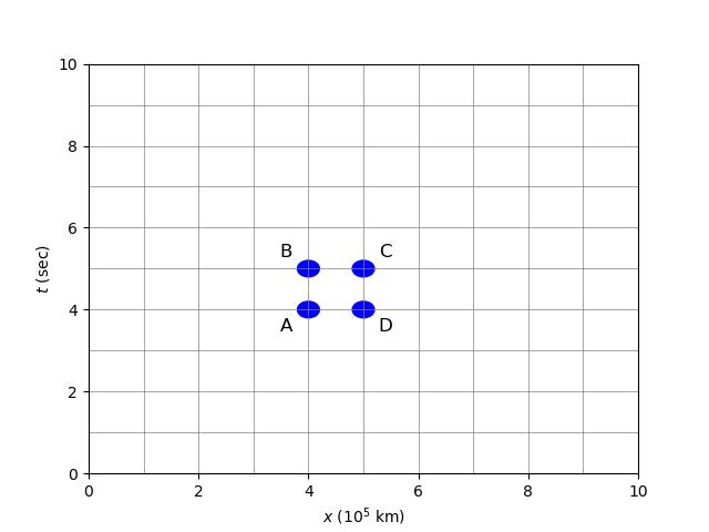Let's consider this rule for the points labeled A, B, C and D in the figure. In this coordinate system, the point labeled by A is also labeled by \(t = 4\) seconds and \(x = 4\times 10^5\) km. Let's calculate the length of a ruler, at rest in this coordinate system, with one end on A and the other end on D, using our invariant distance rule and treating A and D as infinitesimally separated (we'll learn how to deal with finite separations later). A and D both have the same value of the \(t\) coordinate so \(dt = 0\). Their x coordinates differ by \(10^5\) km. So using Eq. \ref{eqn:InvDistMinkowski} we find the length of this ruler is given by \(\sqrt{ds^2} = \sqrt{(10^5 {\rm km})^2} = 10^5\) km.

Box \(\PageIndex{1}\)

Exercise 5.1.1: Use Eq. \ref{eqn:InvDistMinkowski} to find the time that elapses on a clock that freely falls from D to C. Note that in this coordinate system the clock is not moving at all; i.e., its spatial coordinate is not changing value. Show your work. You should find that you get that the time elapsed is 1 second.

Exercise 5.1.2: Consider the points A and C. Is the separation spacelike or timelike? Evaluate, using Eq. \ref{eqn:InvDistMinkowski},  \(\sqrt{-ds^2/c^2}\) if it is timelike and  \(\sqrt{-ds^2/c^2}\) if it is spacelike. What does this mean physically in terms of either a clock or a ruler? Answer with a complete sentence.

You should have seen from these two exercises that the time elapsing on a clock traveling from A to C would be less than 1 second, whereas a "stationary" clock (one at fixed spatial coordinate) traveling from D to C would show 1 second of time elapsed. This is the phenomenon of time dilation you have studied before, often qualitatively summarized with the statement, "moving clocks run slowly."

It may seem cumbersome to use Eq. \ref{eqn:InvDistMinkowski} to calculate the time elapsed on a clock that goes from D to C, or the distance between A and D, when the answers seem obvious. However, we will also use spacetimes where the answers are not so obvious, and we really need the guidance of our invariant distance rule. In general, the coordinate values themselves mean nothing -- they are merely labels. Physical meaning becomes apparent only through use of an invariant distance rule. Keep this in mind.

The physical interpretation of \(ds^2\) may seem a bit complicated. But I think it is stated as simply as it can be. The statement for spacelike separations looks particulary cumbersome. Why do we need to specify something about the speed of the ruler? You might recall that there is a phenomenon called "Lorentz contraction;" i.e., that the length of an object in the direction of its motion depends on its speed. So we do need to specify how the ruler is moving -- and here we do so by specifying the frame in which it is at rest. 

So far we have used nothing of the general theory of relativity -- the above is all from the special theory of relativity which I assume you have already studied. It might be stated in a form you are unfamiliar with. For example we have emphasized the invariant distance and said nothing about Lorentz transformations, and we have restricted ourselves to infinitesimal, rather than finite, invariant distances. The manner of presentation is intentional, as it makes it easy to extend beyond the framework of special relativity, to that of Einstein's general theory.

 

Box \(\PageIndex{2}\)

Exercise 5.2.1: For the spacetime specified by Equation \ref{eqn:InvDistMinkowski}. On a plot of \(x\) vs. \(t\) (what we call a spacetime diagram, like the figure above) draw the trajectory of a particle that is not moving, one that is moving slowly, and then of one that is moving at the speed of light. Place the \(x\)-coordinate on the horizontal axis, as is the usual convention.

 

Principles of the General Theory of Relativity

The general theory of relativity (GR) is a theory of gravitation that is conceptually quite different from the Newtonian theory of gravitation. In the Newtonian theory the motions of objects through space and time are understood as being due to a gravitational force that accelerates them. In GR these motions are understood as resulting from an altered geometry of spacetime, with that geometry determined by the matter/energy distribution.

In the general theory of relativity, it is not in general true that one can label space and time so that the invariant distance rule is given by Eq. \ref{eqn:InvDistMinkowski}, or its generalization to multiple spatial dimensions. In fact, the presence of mass distorts the spacetime so that there is no labeling that will make Eq. \ref{eqn:InvDistMinkowski} true everywhere. However, it is still true in the general theory, like in the special theory, that one can label the spacetime with coordinates, and that their physical meaning is given by a rule specifying the square of the invariant distance between any two infinitesimally-separated points. Further, \(ds^2\) has the same physical interpretation in the general theory as written above.

What do we mean by the geometry of spacetime? That geometry is specified by a rule for the invariant distance that is a function taking in any pair of infinitesimally-separated points and outputting the square of the invariant distance, \(ds^2\). We see above an example of this rule for the special case of a 1+1-dimensional Minkowski spacetime.

How does this geometry dictate how matter moves? For the most part we will only be concerned with the motion of light, which, as we discuss in the next chapter, follows trajectories with \(ds^2 = 0\). More generally, a particularly succinct way of stating the rules of force-free motion is as follows: an object that freely falls from event A to event B does so along a spacetime trajectory that extremizes the time elapsed on a clock traveling with the object. How to convert an extremum principle such as this to equations of motion is presented in the optional A4. Presumably you have seen this before in the case of the action principle of classical mechanics and the resulting Euler-Lagrange equations. We also intend to create an optional A5 with opportunities to practice use of this extremized-time principle in various spacetimes. 

How do matter and energy influence the spacetime geometry? The Einstein Field Equations answer this question; they are beyond the scope of this course. 

 

The Simplest Expanding Spacetime

The invariant distance rule above (Equation \ref{eqn:InvDistMinkowski}) is for a static spacetime. It is appropriate for a spacetime in which there is no matter or energy. If instead we have a spacetime with mass uniformly distributed throughout it, then the geometry would be different; i.e., one could no longer label every point in the spacetime with a value of \(t\) and of \(x\) such that Equation \ref{eqn:InvDistMinkowski} was true. One could however label the spacetime with \(t\) and \(x\) such that this is true:

\[ds^2 = -c^2 dt^2 + a^2(t)dx^2 \label{eqn:InvDistFlatFRW}\]

with \(a(t)\) a function of time. We call \(a(t)\) the "scale factor." The exact behavior of \(a(t)\) depends, as we will see, on both initial conditions and the properties of the material supplying that uniform distribution of mass. If \(\dot a > 0\) the universe is expanding. If \(\dot a < 0\) it is contracting.

This extremely simple model of a spacetime is one with a high degree of relevance to our own. Of course we have three spatial dimensions instead of one, but for calculating some important observables that difference is irrelevant. And also our universe is clumpy; i.e., the distribution of mass is not spatially uniform. However, as emphasized in the Overview chapter, our universe does appear to be highly uniform on large scales and at early times. This model is well worth studying. Let's do that with the following exercises and into the next chapter. 

Box \(\PageIndex{3}\)

Exercise 5.3.1: Imagine a very small ruler instantaneously at rest in the \(x,t\) coordinate system of Equation \ref{eqn:InvDistFlatFRW} at time \(t=t_1\), with one end at location \(x=x_1\) and its other end at \(x=x_1+dx_1\). How long is the ruler?

Box \(\PageIndex{4}\)

Exercise 5.4.1: How much time elapses on a clock on a trajectory of constant \(x\), from \(t=t_1\) to \(t=t_2\) for a spacetime and coordinate system with invariant distances given by Equation \ref{eqn:InvDistFlatFRW}? Hint: you have only been given a rule for infinitesimal separations and this is a finite one. However, you can break up the finite interval into infinitesimal ones and then integrate. 

Box \(\PageIndex{5}\)

Exercise 5.5.1: Still assuming Equation \ref{eqn:InvDistFlatFRW}, draw the paths through spacetime of a pair of particles that are separated from each other and that are not "moving" -- that is, their \(x\) coordinate values are not changing over time. Assume \(a(t)\) is an increasing function of time. What do you notice about the distance between them and how it evolves over time? Be careful not to confuse "distance between them" with the difference in the values of their spatial coordinates.

Exercise 5.5.2: Now, add in the trajectory of a light ray passing from one of these particles to the other. While sketching it out, remember that \(a(t)dx\) is the distance traversed (as measured by an observer at rest in the \(x,t\) coordinate system) as the time coordinate changes by \(dt\), which is the time elapsed as measured by an observer at rest in the \(x,t\) coordinate system. In this \(x\) vs. \(t\) diagram, does light travel in a straight line?

You should have seen in the box above that light does not travel on a straight line in this expanding spacetime as labeled with the \(t\), \(x\) coordinates. This is kind of annoying, and something we will address in the next chapter.

An interesting question to ask about an expanding spacetime is whether the universe ever had, in the past, the scale factor equal to zero. As this would render everything currently in the observable universe all with zero separation between them, this would be quite an extreme situation. Just to get some practice working things out in an expanding spacetime, practice that will be useful later, let's assume \( \dot a = \kappa/a\) for \( \kappa\) some positive constant and see if such a universe ever had \( a = 0\). Let us call the time since \(a = 0\), \(\Delta t\). We can then write

\[ \Delta t = \int dt = \int_0^{a(t)} da/\dot a = \int_0^{a(t)} da (a/\kappa) = a^2(t)/(2\kappa). \]

Since the integral converged, we find that with the assumption given, namely \(\dot a \propto 1/a\), the answer is yes, a finite time in the past the scale factor had the value 0. This is the singularity of the big bang. In such spacetimes we usually choose to call the zero point of time ( \( t = 0\) ), the time when \(a = 0\). [Note that this \( \Delta t\) is the time that would elapse on a stationary clock; i.e., a clock with a fixed spatial coordinate.]

Also note that we made progress with this calculation by replacing \( dt \) with \( dt = da/\dot a \). This is a trick we will use many times to calculate a variety of things.

Another question we can ask is, "how far has light traveled since the beginning." It's interesting because nothing travels faster than the speed of light, so this tells us what the maximum distance is that any signal can propagate. We call this distance the "past horizon." Let's once again assume, for definiteness, \( \dot a = \kappa/a\) and calculate how far light can travel. We know that for light \( ds^2 = 0 \) so we have \(c^2 dt^2 = a^2(t) dx^2\) and therefore \(cdt/a(t) = dx\) so we can write

\[\Delta x = \int dx = \int cdt/a = c\int_0^{a(t)} da/(a \dot a) = \frac{c}{ \kappa} \int _0^{a(t)} da = \frac{c}{ \kappa} a(t)\]

(where you'll note we used the same trick again to convert an integral over time to an integral over the scale factor). Therefore we know the coordinate distance that light has traveled, \( \Delta x\). That coordinate distance corresponds to a physical distance, at time \(t\), of \(a(t) \Delta x = \frac{c}{ \kappa} a^2(t) \).

HOMEWORK Problems

Problem \(\PageIndex{1}\)

Derive the phenomenon of Lorentz contraction using the invariance of the invariant distance. [Do not assume an expanding universe; assume \(ds^2 = -c^2dt^2 + dx^2\)]. The trick to doing this is careful choice of the two events (points in spacetime) for which to calculate their invariant distance. Imagine a ruler moving with respect to an observer at speed \(v\), with the ruler oriented so that it is parallel to the relative velocity. Take event 1 to be when/where the front end of the ruler is at the same spacetime location as the observer, and event 2 to be when/where the back end of the ruler is at the same spacetime location as the observer. By calculating the invariant distance in the observer's rest frame and the ruler's rest frame you should find that the length of the ruler as determined by the observer is \(L' = L/\gamma\) where \(L\) is the length of the ruler in its rest frame.

Problem \(\PageIndex{2}\)

Assume that the scale factore evolves via \( \dot a = \kappa a \) for \( \kappa\) a positive constant. (Note that this is a different assumption than the previous \( \dot a = \kappa/a\) ). Show that in this spacetime the universe never has \( a = 0 \). Do so by showing that the amount of time between \( a = 0 \) and any finite \( a\) is infinite; i.e., show that the appropriate definite integral does not converge.

Problem \(\PageIndex{3}\)

Assume \(ds^2 = -c^2 dt^2 + a^2(t)dx^2\) and once again that \( \dot a = \kappa a \) for \( \kappa\) a positive constant. Our universe appears to be moving asymptotically toward such a case (although except with a 3-dimensional space instead of a 1-dimensional space). Determine what we call the "future horizon." If a light signal is sent out at time \(t_1\) from \(x_1\), in the positive \(x\) direction, to what value of \(x_2\) will it get given an infinite amount of time? The distance between \(x_1\) and \(x_2\) at time \(t_1\), \( a(t_1)(x_2 - x_1)\), is called the future horizon.