
6.1: Overview of Vectors
- Page ID
- 56284

\( \newcommand{\vecs}[1]{\overset { \scriptstyle \rightharpoonup} {\mathbf{#1}} } \)
\( \newcommand{\vecd}[1]{\overset{-\!-\!\rightharpoonup}{\vphantom{a}\smash {#1}}} \)
\( \newcommand{\dsum}{\displaystyle\sum\limits} \)
\( \newcommand{\dint}{\displaystyle\int\limits} \)
\( \newcommand{\dlim}{\displaystyle\lim\limits} \)
\( \newcommand{\id}{\mathrm{id}}\) \( \newcommand{\Span}{\mathrm{span}}\)
( \newcommand{\kernel}{\mathrm{null}\,}\) \( \newcommand{\range}{\mathrm{range}\,}\)
\( \newcommand{\RealPart}{\mathrm{Re}}\) \( \newcommand{\ImaginaryPart}{\mathrm{Im}}\)
\( \newcommand{\Argument}{\mathrm{Arg}}\) \( \newcommand{\norm}[1]{\| #1 \|}\)
\( \newcommand{\inner}[2]{\langle #1, #2 \rangle}\)
\( \newcommand{\Span}{\mathrm{span}}\)
\( \newcommand{\id}{\mathrm{id}}\)
\( \newcommand{\Span}{\mathrm{span}}\)
\( \newcommand{\kernel}{\mathrm{null}\,}\)
\( \newcommand{\range}{\mathrm{range}\,}\)
\( \newcommand{\RealPart}{\mathrm{Re}}\)
\( \newcommand{\ImaginaryPart}{\mathrm{Im}}\)
\( \newcommand{\Argument}{\mathrm{Arg}}\)
\( \newcommand{\norm}[1]{\| #1 \|}\)
\( \newcommand{\inner}[2]{\langle #1, #2 \rangle}\)
\( \newcommand{\Span}{\mathrm{span}}\) \( \newcommand{\AA}{\unicode[.8,0]{x212B}}\)
\( \newcommand{\vectorA}[1]{\vec{#1}} % arrow\)
\( \newcommand{\vectorAt}[1]{\vec{\text{#1}}} % arrow\)
\( \newcommand{\vectorB}[1]{\overset { \scriptstyle \rightharpoonup} {\mathbf{#1}} } \)
\( \newcommand{\vectorC}[1]{\textbf{#1}} \)
\( \newcommand{\vectorD}[1]{\overrightarrow{#1}} \)
\( \newcommand{\vectorDt}[1]{\overrightarrow{\text{#1}}} \)
\( \newcommand{\vectE}[1]{\overset{-\!-\!\rightharpoonup}{\vphantom{a}\smash{\mathbf {#1}}}} \)
\( \newcommand{\vecs}[1]{\overset { \scriptstyle \rightharpoonup} {\mathbf{#1}} } \)
\(\newcommand{\longvect}{\overrightarrow}\)
\( \newcommand{\vecd}[1]{\overset{-\!-\!\rightharpoonup}{\vphantom{a}\smash {#1}}} \)
\(\newcommand{\avec}{\mathbf a}\) \(\newcommand{\bvec}{\mathbf b}\) \(\newcommand{\cvec}{\mathbf c}\) \(\newcommand{\dvec}{\mathbf d}\) \(\newcommand{\dtil}{\widetilde{\mathbf d}}\) \(\newcommand{\evec}{\mathbf e}\) \(\newcommand{\fvec}{\mathbf f}\) \(\newcommand{\nvec}{\mathbf n}\) \(\newcommand{\pvec}{\mathbf p}\) \(\newcommand{\qvec}{\mathbf q}\) \(\newcommand{\svec}{\mathbf s}\) \(\newcommand{\tvec}{\mathbf t}\) \(\newcommand{\uvec}{\mathbf u}\) \(\newcommand{\vvec}{\mathbf v}\) \(\newcommand{\wvec}{\mathbf w}\) \(\newcommand{\xvec}{\mathbf x}\) \(\newcommand{\yvec}{\mathbf y}\) \(\newcommand{\zvec}{\mathbf z}\) \(\newcommand{\rvec}{\mathbf r}\) \(\newcommand{\mvec}{\mathbf m}\) \(\newcommand{\zerovec}{\mathbf 0}\) \(\newcommand{\onevec}{\mathbf 1}\) \(\newcommand{\real}{\mathbb R}\) \(\newcommand{\twovec}[2]{\left[\begin{array}{r}#1 \\ #2 \end{array}\right]}\) \(\newcommand{\ctwovec}[2]{\left[\begin{array}{c}#1 \\ #2 \end{array}\right]}\) \(\newcommand{\threevec}[3]{\left[\begin{array}{r}#1 \\ #2 \\ #3 \end{array}\right]}\) \(\newcommand{\cthreevec}[3]{\left[\begin{array}{c}#1 \\ #2 \\ #3 \end{array}\right]}\) \(\newcommand{\fourvec}[4]{\left[\begin{array}{r}#1 \\ #2 \\ #3 \\ #4 \end{array}\right]}\) \(\newcommand{\cfourvec}[4]{\left[\begin{array}{c}#1 \\ #2 \\ #3 \\ #4 \end{array}\right]}\) \(\newcommand{\fivevec}[5]{\left[\begin{array}{r}#1 \\ #2 \\ #3 \\ #4 \\ #5 \\ \end{array}\right]}\) \(\newcommand{\cfivevec}[5]{\left[\begin{array}{c}#1 \\ #2 \\ #3 \\ #4 \\ #5 \\ \end{array}\right]}\) \(\newcommand{\mattwo}[4]{\left[\begin{array}{rr}#1 \amp #2 \\ #3 \amp #4 \\ \end{array}\right]}\) \(\newcommand{\laspan}[1]{\text{Span}\{#1\}}\) \(\newcommand{\bcal}{\cal B}\) \(\newcommand{\ccal}{\cal C}\) \(\newcommand{\scal}{\cal S}\) \(\newcommand{\wcal}{\cal W}\) \(\newcommand{\ecal}{\cal E}\) \(\newcommand{\coords}[2]{\left\{#1\right\}_{#2}}\) \(\newcommand{\gray}[1]{\color{gray}{#1}}\) \(\newcommand{\lgray}[1]{\color{lightgray}{#1}}\) \(\newcommand{\rank}{\operatorname{rank}}\) \(\newcommand{\row}{\text{Row}}\) \(\newcommand{\col}{\text{Col}}\) \(\renewcommand{\row}{\text{Row}}\) \(\newcommand{\nul}{\text{Nul}}\) \(\newcommand{\var}{\text{Var}}\) \(\newcommand{\corr}{\text{corr}}\) \(\newcommand{\len}[1]{\left|#1\right|}\) \(\newcommand{\bbar}{\overline{\bvec}}\) \(\newcommand{\bhat}{\widehat{\bvec}}\) \(\newcommand{\bperp}{\bvec^\perp}\) \(\newcommand{\xhat}{\widehat{\xvec}}\) \(\newcommand{\vhat}{\widehat{\vvec}}\) \(\newcommand{\uhat}{\widehat{\uvec}}\) \(\newcommand{\what}{\widehat{\wvec}}\) \(\newcommand{\Sighat}{\widehat{\Sigma}}\) \(\newcommand{\lt}{<}\) \(\newcommand{\gt}{>}\) \(\newcommand{\amp}{&}\) \(\definecolor{fillinmathshade}{gray}{0.9}\)Basic Vector Definition
What we are really interested in now is describing how objects move. A very useful tool that will help us achieve this goal is the concept of a vector. We can give a definition of a vector as something that exhibits both direction and magnitude. This concept might appear abstract at first, but as we begin to use the vectors in different contexts, we will develop a deeper and richer understanding. Remember how hard it was to define energy. Our understanding of energy continually increased as we applied the idea to multiple physical phenomena. Similarly with vectors, even though we currently give it a short one-sentence definition, understanding comes as we use the concept and work with it over the remainder of this and the next two chapters.
In Physics 7A we were only concerned with magnitudes of quantities, such as speed and mass of an object which was sufficient information to calculate its kinetic energy. However, if you want to know precisely where in space a moving object will be after some time, in addition to speed, we also need to know its direction. The velocity of an object is a vector quantity which describes both its speed (magnitude of the velocity vector) and its direction. One example where the velocity is important to know is when two objects are interacting. Two moving objects colliding head-on compared to two moving objects colliding while moving in the same direction will yield very different outcomes, even if their speeds are the same in both scenarios. We will explore such interaction when we discuss conservation of momentum in the next chapter. Force is another quantity where both the magnitude (how strong is the push or pull) and then direction (in which direction is the push or pull) will matter to explain how an object will react under the influence of forces. For example, two people pushing the table with the same strength in the same direction will result in different dynamics (the table will move most likely) compared with the same strength is applied in opposite directions (the table will not budge). Acceleration is another useful vector quantity which describes the rate of change of velocity and is directly related to the forces acting on an object. We will explore the effects of forces in much greater details in this and the following chapters.
Vector Representation
One way to represent vectors is with arrows pointing in the direction of the vector, where the length of the arrow represents the magnitude of the vector. It is only the relative lengths of various arrows that matter, there is not rule that says that a specific length represents a specific magnitude. For example, if we choose a length of 1 cm to represent a velocity vector with a speed of 10 m/s, then another velocity vector whose length is double, 2 cm, will represent a speed of 20 m/s. We refer to the arrowhead as the head of the vector, and the other end as the tail.
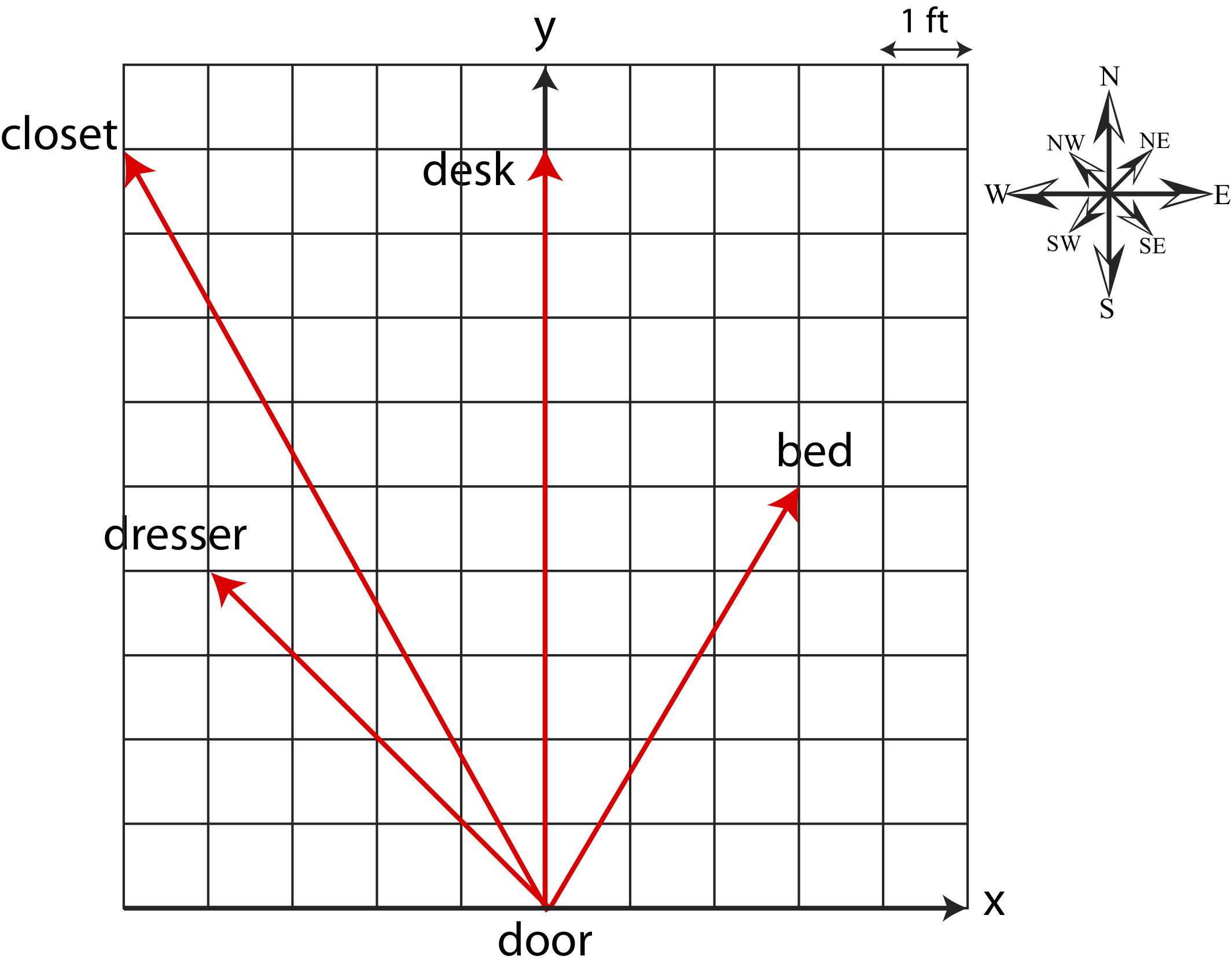
Let us explore vector representation in the context of a position vector, since it is perhaps the simplest vector quantity to apply to every day experience. A position vector describes the location of an object relative to some point of reference. If you are trying to describe the layout of your bedroom to your friend, you can use the door as the reference point, or the origin, of the position vectors which will represent the locations of objects in your room. It is not sufficient to say that your desk is 9 feet away from the door. Your friend will not know on which side of the room the desk located. Thus, to describe the position of your desk exactly, you need a vector quantity to specify that your desk is 9 feet straight from the door. Rather then using "straight", "right" or "left", it is more convenient to use the x-y coordinate system. Figure 6.1.1 below shows a set of position vectors to the center of objects in a bedroom, where each grid square is one foot in distance. In the figure the positive x-direction is to the right of the door, the negative x-direction is to the rest, the positive y-direction is straight ahead, and the negative y-direction is straight behind. We will often use compass coordinates as well to describe direction: in Figure 6.1.1 "north" represents straight from the door, east to the right, and west to the left.
These vectors are two-dimensional since we are only concerned with where the various objects are located on the floor. If we also represented the height of each object, then we would have to describe the vector in three-dimensions. For example, the bed is 5 feet straight, 3 feet to the right, and 2 feet up from the floor. For now, we will mostly focus on two-dimensional vectors.
Figure 6.1.1: Position Vectors
In print, a small arrow is put over the symbol to represent a vector. For example, force, position, velocity, and acceleration vectors are represented as \(\vec F, \vec r, \vec v\), and \(\vec a\). In this book we will stick to this notation, but in other text you might encounter a bold symbol for vector notation (such as F, r, v, a).
Vectors are represents by their components, which are the values of the vectors in each of the spacial direction. For example, the position vector of the desk in Figure 6.1.1 has a component of 0 ft in the x-direction and of 9 ft in the positive y-direction. To write down the values of the vectors we will use the following notation: \(\vec A=(A_x,A_y,A_z)\), where the values in the parenthesis are the vector components. Note, the vector components can be either zero, positive, or negative depending in which quadrant the vector lies in. The position vector for the desk is then written as, \(\vec r_{\textrm{desk}}=(0,9)\) ft since it is precisely on 9 feet in the positive y-direction. The dresser's position vector is \(\vec r_{\textrm{dresser}}=(-4,4)\) ft since it is four feet from the door in the negative x-direction and four feet from the door in the +y direction. Note, we have dropped the the z-component all together from the position vectors in this room, since for this particular situation we are only concerned with the x-y position of the objects and not their heights. Thus, the z-component is always zero in this particular description of position of objects.
This notation of the position vector, \(\vec r\), fully describes the location of objects from the door, which is defined as the origin for all position vectors. But this is not the only way to represent the position vector. One can also do it by using the magnitude (the distance form the door to the object) and the direction. For example, the desk is a distance of 9 feet in the positive y-direction (or north) from the door. The notation for magnitude of a vector \(\vec A\) is \(|\vec A|\), or sometimes you will encounter simply, \(A\), without the arrow over it to specify magnitude. Thus, either writing \(\vec r_{\textrm{desk}}=(0,9)\) or \(|\vec r_{\textrm{desk}}|=9\) ft pointing north are equivalent ways of describing the position vector of the desk.
One way to represent the position vector of the bed is by components, \(\vec r_{\textrm{bed}}=(3,5)\) ft. But how do we describe it by using magnitude and direction? We need to know how far the bed is from the door, we cannot simply count the squares in Figure 6.1.1 and get an exact answer. Using a ruler is one way to do it, but there is a more accurate calculation that can be done as described shortly. Also, simply stating its direction as northeast or above the +x axis is not accurate, since it only specifies the first quadrant but not the bed's exact location. Thus, we need to both calculate the distance and to specify the exact angle the vector makes with the +x axis. To do so we need to turn to trigonometry. Consider the figure below which depicts some vector \(\vec A\) with components \(A_x\) and \(A_y\), \(\vec A=(A_x,A_y)\).
Figure 6.1.2: Vector Components
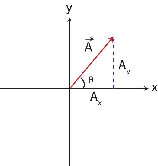
The magnitude (length) of the vector makes a right triangle with the two components of the vector, where the magnitude is the hypotenuse. Thus, to find the magnitude of the vector \(\vec A=(A_x,A_y)\) we can use the Pythagorean theorem:
\[|\vec A|=\sqrt{A^2_x+A^2_y} \label{mag}\]
To find the angle, \(\theta\) shown in the figure above, we can use the property of a tangent:
\[\theta =\arctan\Big(\big\lvert\frac{A_y}{A_x}\big\rvert\Big)\label{angle}\]
We use the absolute value symbol in Equation \ref{angle} since we want to describe the direction by stating the angle between \(0^{\circ}\) and \(90^{\circ}\), and then by specifying the quadrant either by stating, for example, the vector points "down from the negative x-axis" or using the compass coordinate "southwest". Thus, even if the x- or y- components are negative you should use the absolute values of these components when calculating the angle.
Returning to the position vector of the bed, \(\vec r_{\textrm{bed}}=(3,5)\) ft, we can now use the trigonometric properties, described above, to represent the vector with its magnitude \(|\vec r_{\textrm{bed}}|=\sqrt{3^2+5^2}=5.83\) ft and angle of \(\theta =\arctan\Big(\frac{5}{3}\Big)=59^{\circ}\) above the positive x-axis or pointing northeast. The position vector of the closet, \(\vec r_{\textrm{closet}}=(-5,9)\) ft has magnitude of \(|\vec r_{\textrm{bed}}|=\sqrt{5^2+9^2}=10.3\) ft and direction of \(\theta =\arctan\Big(\frac{9}{5}\Big)=60.9^{\circ}\) above the negative x-axis or pointing northwest.
You might be wondering why one should bother to express the vector in terms of magnitude and direction direction since expressing the vectors in Figure 6.1.1 directly in terms of components is simpler, you can read the values of the x- and y- components directly from the figure using the provided grid and scale. However, sometime information for a vector quantity is provided or measured directly in terms of magnitude and direction. And it is also more intuitive to picture the location of a bed if one gave you the information in terms distance and angle from the door rather than in terms of components. In other words, instead of measuring directly that the closet is 5 feet east and 9 feet north from the door, you may have measured with a ruler the distance of 10.3 feet from the door and with a protractor an angle of \(60.9^{\circ}\) above the negative x-axis. Having this information does describe the vector completely, but it is still often very useful to represent in terms of its components, as we will see shortly below when discussing adding and subtracting vectors. We can find the components from the magnitude \(|\vec A|\) and direction \(\theta\) plus quadrant, by using trigonometry once again. From Figure 6.1.2 using the definition of sine and cosine the x- and y- components of the vector in terms of magnitude and angle are given by:
\[A_x=|\vec A|\cos\theta\]
\[A_y=|\vec A|\sin\theta\]
Let us check that these equations give us the correct components for the closet's position vector, if you were just told that the closet is 10.3 feet away from the door and at an angle of \(60.9^{\circ}\) northwest. Using the equation above and noting that "northwest" implies that the the x-component will be negative and the y-component positive we find that, \(r_x=-(10.3~\textrm{ft}) \cos 60.9^{\circ}=-5~\textrm{ft}\) and \(r_y=(10.3~\textrm{ft}) \sin 60.9^{\circ}=9~\textrm{ft}\), resulting \(\vec r_{\textrm{closet}}=(-5,9)~\textrm{ft}\) as expected.
Adding and Subtracting Vectors
As we introduce new models in the following chapters, we will see multiple applications where we will need to add or subtract vectors. Adding vectors is not as trivial as adding scalar quantities. We know that the combined mass of a 2kg and a 3kg objects is 5kg. But we cannot simply add magnitudes of vectors together to obtain the magnitude of combined vectors. This method would only work if the two vectors point in the same direction. For example, if you walk 2 feet north and then walk 3 more feet also north, the combined vector (which represents walking directly from the start to end) is indeed the sum of the magnitudes pointing in the same direction, 5 feet north. However, let us look at another example as depicted in the figure below.
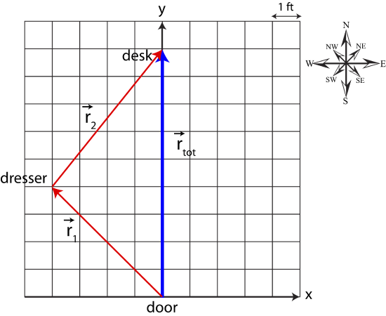
In this scenario, you walk to your dresser first, and then to your desk. This is equivalent to walking to your desk directly, 9 feet north. But 9 feet is clearly a shorter distance than the distance to get to the dresser plus the distance to walk to the desk. Thus, we cannot simply add magnitudes of the position vectors \(\vec r_1\) and \(\vec r_2\) in Figure 6.1.2.
Our goal is to come up with a method such that adding the position vector to the dresser, \(\vec r_1\), with the position vector from the dresser to the desk, \(\vec r_1\), gives us the position vector directly to the desk, here defined as \(\vec r_{tot}\) and represented by the bolder blue arrow in Figure 6.1.2: \(\vec r_{tot}=\vec r_1+\vec r_2\). Let us represent the vectors by components. The position vector to the dresser is \(\vec r_1=(-4,4)\). When representing \(\vec r_2\) we have to remember that all position vectors are defined relative to the origin (0,0) defined at the location of the door. Thus, although the tail of the vector is at the location of the dresser, it must be respresented relative to the origin. You can always take the vector \(\vec r_2\) and move it to the location of the door (origin) preserving the length and direction of the vector. From figure 6.1.2, you can simply count the number of squares in the x- and y- directions starting from the tail of \(\vec r_2\), resulting in \(\vec r_2=(4,5)\). The total vector, directly to the desk is \(\vec r_{tot}=(0,9)\). You can see from the components of \(\vec r_1\) and \(\vec r_2\) that to obtain the components of the total vector, you need to sum the x-components, \(\vec r_{tot,x}=-4+4=0\), to get the x-component of the total vector, and likewise you need to sum the y-components, \(\vec r_{tot,y}=4+5=9\). Mathematically, the sum of two vectors is written as:
\[\vec A_{tot}=\vec A_1+\vec A_2=(A_{1,x}+A_{2,x},A_{1,y}+A_{2,y})\]
To obtain the magnitude and direction of the total vector, you can use Equations \ref{mag} and \ref{angle}.
You can also see from Figure 6.1.2 that the tail of \(\vec r_2\) is positioned at the head of \(\vec r_1\), and the sum of the two vectors, \(\vec r_{tot}\), is positioned such that its tail is at the tail of \(\vec r_1\) and its head is at the head of \(\vec r_2\). This describes the geometric method of vector addition, known as the head-to-tail method. Take three vectors shown in Figure 6.1.3 and move them such that the head of one vector touches the tail of the next one as shown on the right figure. The resultant vector, \(\vec r_{tot}\) is drawn from the tail of the first vector to the head of the last vector as shown.
Figure 6.1.3: Head-to-Tail Method for Vector Addition
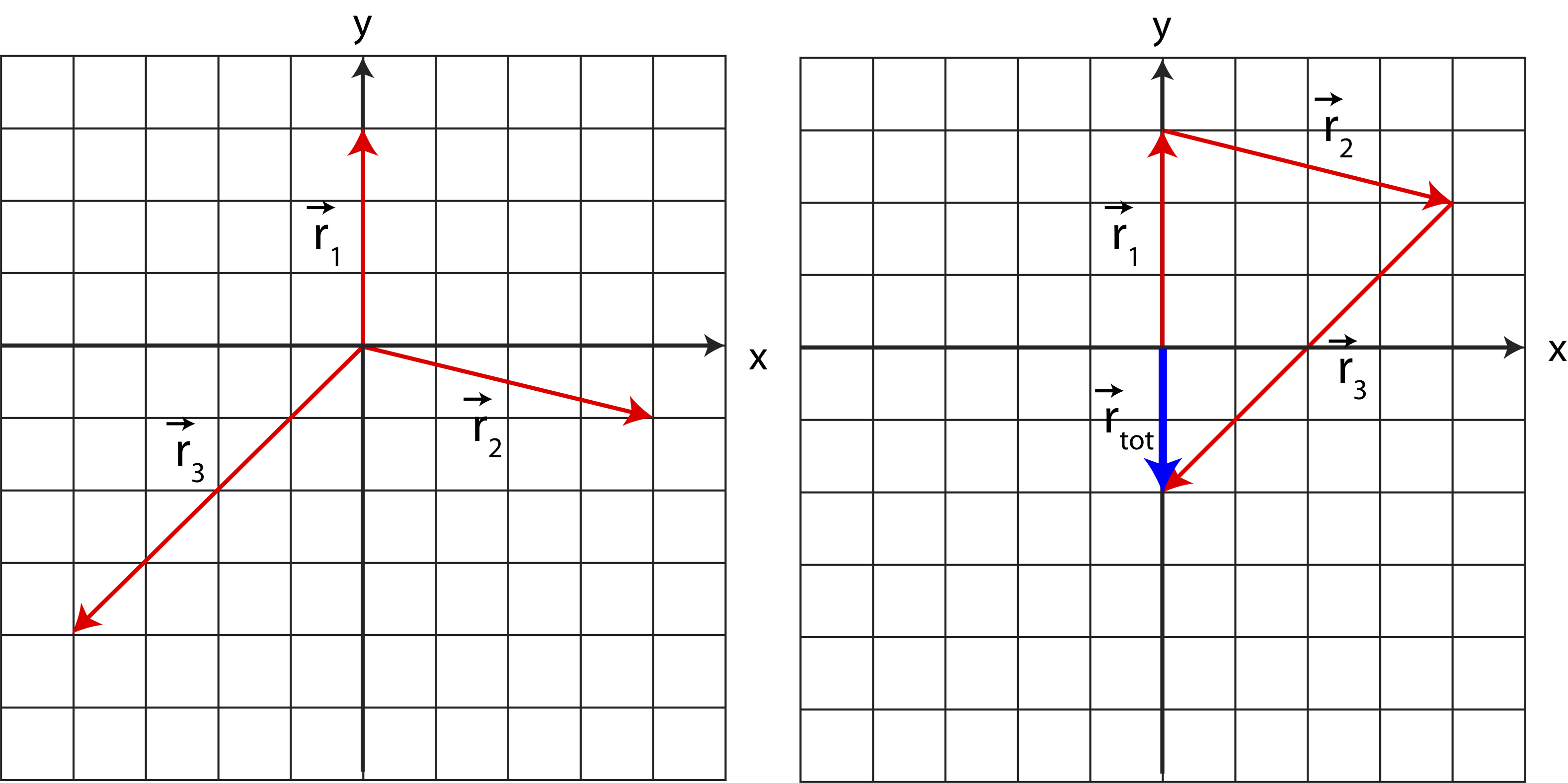
To check this method, let us sum the three vectors by components:
\[\vec r_{tot}=\vec r_{1}+\vec r_{2}+\vec r_{3}=(0,3)+(4,-1)+(-4,-4)=(0+4-4,3-1-4)=(0,-2),\]which is exactly the vector \(\vec r_{tot}\) drawn in Figure 6.1.3.
Example \(\PageIndex{1}\)
An apple tree is positioned 3 meters away from you pointing \(50^{\circ}\) southwest. And orange tree is is positioned 6.5 meters away from the apple tree, in the direction of \(25^{\circ}\) pointing southeast from the apple tree. If you were to walk directly from your location to the orange tree, how far should you walk an in which direction (angle and compass direction)?
- Solution
-
It is often much easier to solve problems that involve vector algebra if you first draw then out, if they are not drawn for you already. The figure below depicts the information provided in the problem.
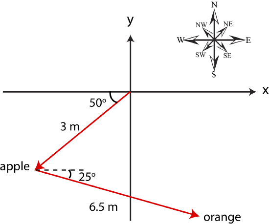
Now you can see that the vector from the origin (your position) directly to the orange tree will point southeast and will have a magnitude somewhere between 3 and 6.5 meters. In order to find the vector to the orange tree, we need to add the vector from the origin to the apple tree with the vector from the apple to the orange tree. To do so, we first need to express both vectors in terms of their components, then add them by components, and finally calculate the magnitude and angle of the vector resulting from this addition.
The apple tree's position vector\(\vec r_a\) in terms of components is:
\[\vec r_a=|\vec r_a|(-\cos\theta,-\sin\theta)=3 m(-\cos 50^{\circ},-\sin 50^{\circ})=(-1.93,-2.30) m\]
The orange tree's position vector\(\vec r_o\) is:
\[\vec r_o=|\vec r_o|(\cos\theta,-\sin\theta)=6.5 m(\cos 25^{\circ},-\sin 25^{\circ})=(5.89,-2.75) m\]
The sum of the two vectors \(\vec r_{tot}\) is:
\[\vec r_{tot}=\vec r_{a}+\vec r_{o}=(-1.93+5.89,-2.30-2.75)=(3.96,-5.05)\]
Magnitude of \(\vec r_{tot}\) is:
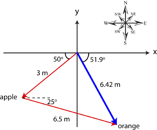
\[|\vec r_{tot}|=\sqrt{3.96^2+5.05^2}=6.42 m\]
Angle is:
\[\theta=\arctan\Big (\frac{5.05}{3.96}\Big )=51.9^{\circ} \]
in the southeast direction.
You can see the vector \(\vec r_{tot}\) represented by the thick blue arrow in the figure below.
To subtract two or more vectors, we use a very similar method as adding vectors. As for scalar addition, the same principle applies: the difference between two numbers is just the sum of one number plus the negative of another one: \(a-b=a+(-b)\). Likewise, for vectors, \(\vec a-\vec b=\vec a+(-\vec b)\). To negate a vector \(\vec A\) you need to negative each component of that vector: \(-\vec A=(-A_x,-A_y)\). This means that the direction of the vector flips by \(180^{\circ}\) when you negate a vector. For example a vector \(\vec A=(4,3)\) has a magnitude of 5 and points northeast at \(53.1^{\circ}\) from the positive x-axis. The negative of this vector \(-\vec A=(-4,-3)\) still has the same magnitude of 5, but now points southwest with an angle of \(53.1^{\circ}\) below the negative x-axis, so \(-\vec A\) is just \(\vec A\) rotated by \(180^{\circ}\). Therefore, to subtract vectors geometrically, you need to flip the vector(s) being subtracted by \(180^{\circ}\), and then apply the usual head-to-tail method for addition. To subtract vectors by components, you simply need to subtract each component individually:
\[\vec A_1-\vec A_2=(A_{1,x}-A_{2,x},A_{1,y}-A_{2,y})\]
In the next few chapters we will focus on analyzing motion of objects. One important property of a moving object is its displacement, a vector quantity which describes both the distance by which an object moved in some interval and the direction in which it moved. If the initial position of an object is some location A and its final position is another location B, displacement vector points from A to B.
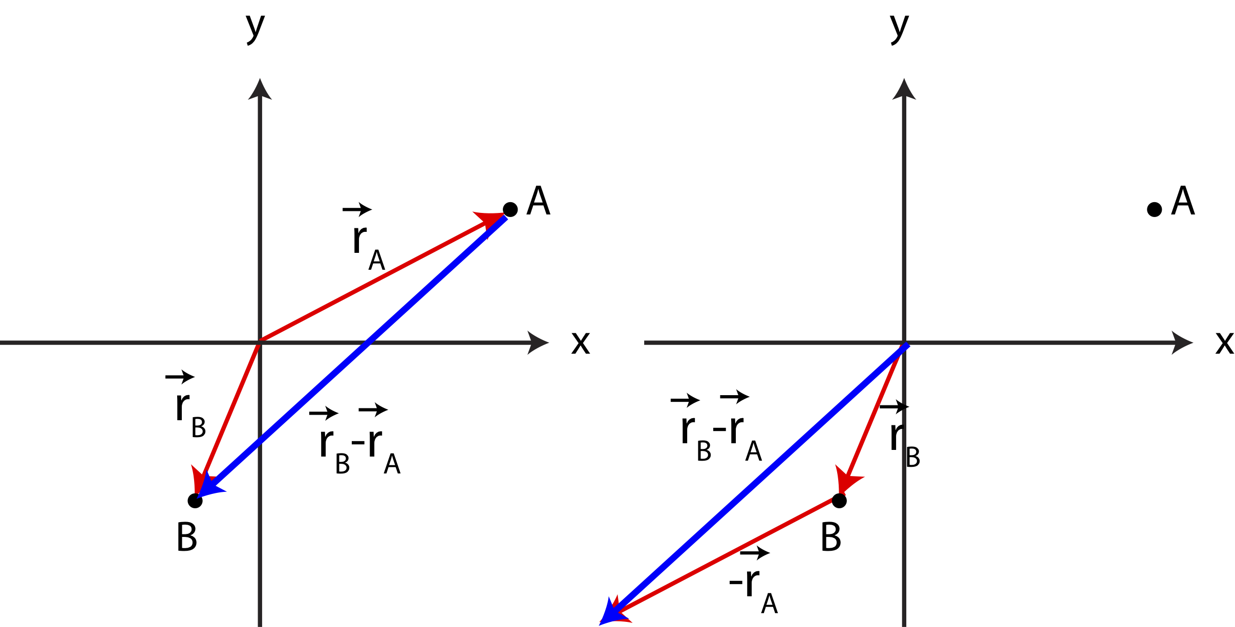
Figure 6.1.4 below shows two locations A and B, described by position vectors \(\vec r_A\) and \(\vec r_B\), respectively. If an object changed its position from point A to B, then the displacement vector is \(\Delta\vec r_{AB}\equiv\vec r_B-\vec r_A\), as drawn pointing from A to B. The right side of the figure depicts the head-to-tail method for obtaining \(\Delta\vec r_{AB}\) from the two position vectors. Vector \(\vec r_A\) is flipped \(180^{\circ}\), and its tail is placed at the head of \(\vec r_B\). The summation vector pointing from the tail of \(\vec r_B\) to the head of \(-\vec r_A\) represents the displacement vector \(\vec r_B-\vec r_A\). Note, two vectors are equivalent as long as their magnitude and direction is the same, so you can see, by eye, that the displacement vectors in both figures look the same.
Figure 6.1.4: Displacement Vector
Generally, the displacement vector represents a vector which points from some initial position, \(i\), to a final position \(f\):
\[\Delta\vec r\equiv\vec r_f-\vec r_i\]
Example \(\PageIndex{2}\)
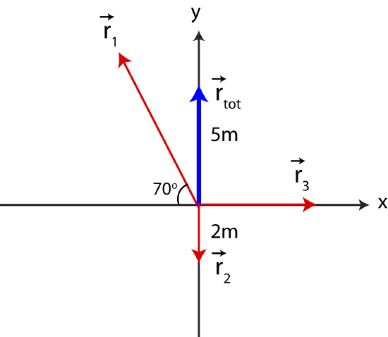
Three position vectors are added resulting in a net vector pointing north with a magnitude of 5 meters. The first vector points northwest at \(70^{\circ}\), the second vector points south and has a magnitude of 2m, and the third vector points east. Find the magnitude of the third vector.
- Solution
-
The graph below depicts the provided information.
The three vectors add up to the total vector:
\[\vec r_{tot}=\vec r_{1}+\vec r_{2}+\vec r_{3}=(-|\vec r_{1}|\cos 70^{\circ}+r_{3,x},|\vec r_{1}|\sin 70^{\circ}-2)=(0,5)\]
Let us split the equation above in terms of components:
\[r_{tot,x}=-|\vec r_{1}|\cos 70^{\circ}+r_{3,x}=0\]
\[r_{tot,y}=|\vec r_{1}|\sin 70^{\circ}-2=5\]
Looking at the equation above, we can first solve for the magnitude of \(\vec r_1\) using the y-components since that's the only unknown in the y-direction, and then use the result to solve for the magnitude of \(\vec r_3\).
Solving for the magnitude of \(\vec r_1\):
\[|\vec r_{1}|=\frac{3}{\sin 70^{\circ}}=3.19m\]
Now plugging in this result in the equation in the x-direction and solving for \(r_{3x}\):
\[r_{3x}=3.19\cos 70^{\circ}=1.09 m\]
Since the vector \(\vec r_{3}\) only has a component in the x-direction, its magnitude is just its x-component: \(|\vec r_{3}|=r_{3x}=1.09 m\).
Velocity and Acceleration Vectors
We just defined the displacement vector which is a vector representing the change in position as an object moves from an initial to a final location. The velocity vector will give us additional information, specifically how fast the object is moving in the direction of displacement. Since the velocity of the object does not need to be constant, we define the average velocity, \(\vec v_{avg}\), which is the average rate of displacement, \(\Delta\vec r\), over time, \(\Delta t\), that it took to move from the initial to final state:
\[\vec v_{avg}=\frac{\Delta\vec r}{\Delta t}\]
A given motion may cover a lot of distant and takes a long time, there could be a lot of variation in both speed and direction of motion between the initial and final locations, so a lot of information might be missing from knowing only the average velocity. Therefore, it is also useful to define instantaneous velocity, \(\vec v\), over some small time period \(dt\):
\[\vec v=\lim_{\Delta t\rightarrow 0}\frac{\Delta\vec r}{\Delta t}=\frac{d\vec r}{dt}\label{v-inst}\]
Figure 6.1.5 below shows an example of a path you take marked by a dashed line to move from location A to B to C. It is important to realize that displacement vector does not describe a particular path an object takes to move between two locations, but it is a vector which points from some initial location to a final location, regardless of the path taken to move between the two locations.
Figure 6.1.5: Displacement Example
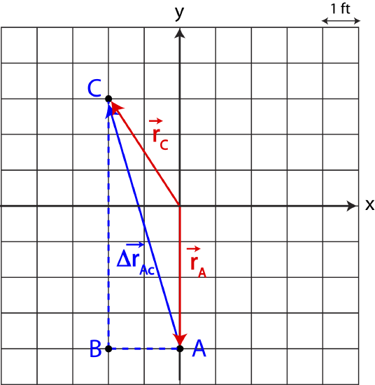
In the example depicted in Figure 6.1.5, even though the path is described by the dashed lines, the displacement vector, \(\Delta\vec r_{AC}=\vec r_C-\vec r_A\), points directly from A to C. Reading from the grid we find by subtracting the two position vectors that \(\Delta\vec r_{AC}=(-2,3)-(0,-4)=(-2,7)~\textrm{ft}\), which is the same result you could obtain by simply reading the components of the displacement vector directly from the graph. If the entire path took 60 seconds to complete, then the average velocity would be:
\[\vec v_{avg}=\frac{\Delta\vec r_{AC}}{\Delta t}=\frac{(-2,7)}{60}\frac{\textrm{ft}}{\textrm{sec}}\]
Note, when you divide or multiple a vector by a constant, you simply need to divide or multiple each component by that constant, so \(\vec v_{avg}=(-1/30,7/60)~\textrm{ft/sec}\). The average speed is the magnitude of the velocity vector resulting in \(v_{avg}=0.121\) ft/sec, and the angle is calculated to be \(\theta=74.1^{\circ}\) in the northwest direction. Although, you never take the path directly in the northwest direction, this is just the average velocity over the entire path.
Knowing the average velocity as calculated above does not give us any information about the specific path that you took to get from location A to C. Let us assume that on your journey between locations A and B you were walking with a constant speed and it took 15 seconds to cover the distance between A and B. This information allows us to compute your instantaneous velocity between points A and B, \(\vec v= (-2/15,0)\) ft/sec, which tells us that you moved at a speed of 0.133 ft/sec in the west direction during that portion of the path. If the profile of your motion is not described by a simple constant speed and a straight line direction, but rather given by some curve, you would need to use the derivative definition of instantaneous velocity given in Equation \ref{v-inst}.
Another important vector quantity that we will discuss in greater detail in later chapters is acceleration which describes the rate of change of velocity. If the motion is at a constant speed and in a straight line (no change in direction), the the acceleration is zero. However, if the speed and/or direction are changing then the object will experience non-zero acceleration which we will relate to forces acting on the object in the next section. Like for velocity, we can define an average acceleration as the rate of change of velocity from some initial velocity, \(\vec v_i\) , to a final velocity, \(\vec v_f\), over a time period, \(\Delta t\):
\[\vec a_{avg}=\frac{\Delta\vec v}{\Delta t}\]
The average velocity does not tell us about variations of changes in velocity between the intial and final times. So instantaneous acceleration is sometimes a more useful quantity to define:
\[\vec a=\lim_{\Delta t\rightarrow 0}\frac{\Delta\vec v}{\Delta t}=\frac{d\vec v}{dt}\]
Alert
When an object is accelerating, in every day language, it is interpreted as the object is speeding up. In physics, the proper definition of acceleration is the rate of change of velocity. This means that when acceleration is not zero, the object can be either speeding up, slowing down, or changing direction. Often the word "deceleration" is used to describe the act of slowing down, but in physics we will always refer to any kind of velocity change as "acceleration".