1.1: Vectors

Definition of a Vector

Just being able to put numbers on physical quantities is not sufficient for describing nature. Very often physical quantities have directions. For example, a description of something’s motion is incomplete if you merely state how fast it is going. [Okay, so an asteroid is moving at 35,000 miles per hour, but is it headed for Earth?!] We therefore have the following definition for physical quantities that exhibit both these properties:

Definition: Vector

A vector is a quantity with both magnitude and direction.

We will frequently represent a vector quantity with an arrow, where the direction of the vector is the direction that the arrow points, and the magnitude of the vector is represented by the length of the arrow. This is not to say that vectors are arrows – arrows just make a handy geometric representation. So while an arrow representing a vector might be 6cm long, that doesn’t mean that the vector has a magnitude of 6cm. The vector might represent the speed and direction of a moving object, for example, and then the vector’s magnitude isn’t even in units of cm. However, if we draw two arrow representations of the same sort of quantity, and one is twice as long as the other, the implication is that the longer arrow represents a vector with twice the magnitude of the vector represented by the shorter arrow.

Alert

There is no way to compare magnitudes of different physical quantities. If a distance vector is drawn as an arrow on the same page as a velocity vector’s arrow, the relative sizes of the two arrows are meaningless.

There are a few other things that we should say about vectors and the arrows that represent them:

• Where the arrow representing a vector is positioned is not a distinct feature of the vector. That is, an arrow representing a vector can be moved at will, and so long as it isn’t stretched, shrunk, or rotated, it will represent the same vector. Just changing an arrow's location does not change its magnitude or its direction if it is moved carefully.
• Vector directions (and therefore the directions of their representative arrows) can be reversed mathematically through multiplication by –1.
• Vector lengths can be expanded or shrunk (scaled) through multiplication by a regular number (called a scalar). If the number is greater than 1, the vector expands in length, and if it is less than 1, it contracts.

One other thing... When we write a symbol for a vector quantity, we will do so with a small arrow above the letter, like this: \(\overrightarrow A\). Variables with the same letter as a defined vector that do not include an arrow, are assumed to represent the magnitude of that vector. So for example, when used in the same context, the variable A represents the magnitude of \(\overrightarrow A\).

Vector Addition/Subtraction

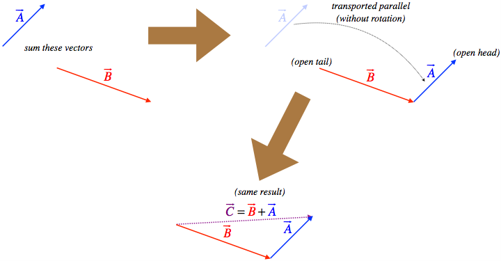
For these mathematical quantities we call vectors to have any value to us, they have to allow for simple mathematical operations, such as addition. The directional nature of vectors makes addition much trickier than simply summing the two magnitudes. It turns out that a well-defined vector addition involves simple geometry. It goes like this: Transport one of the vectors (in a parallel fashion, so as not to change its direction) so that its tail is in contact with the head of the other vector. Then fashion a new vector such that its tail is at the open tail and its head is at the open head.

Figure 1.1.1 – Graphical Vector Addition

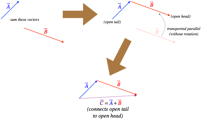
Figure 1.1.2 – Vector Addition is Commutative

What about subtracting two vectors? Well, we can do this by following the same method as for regular numbers: Whichever vector we wish to subtract we multiply by –1, and then add the result to the other vector, which we do in the manner described above. We already know that multiplying a vector by –1 reverses its direction (and leaves its magnitude unchanged), so this is a well-defined operation for us.

Vector Components

The graphical method of adding vectors are not always convenient. For example, we shouldn’t have to actually measure the length of the new vector, we should be able to calculate it. Well, of course we can do this using some sophisticated knowledge of triangles. For example, given we know the lengths and directions of the two vectors we are adding, we can determine the length of the third leg of the triangle using the Law of Cosines:

\[ C^2 = A^2 + B^2 -2AB \cos \theta\]

With all of the lengths of the triangle legs and one of the angles (the one between \(A\) and \(B\)), we can get the other angles using the Law of Sines.

Exercise

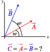
The magnitudes of the two vectors shown in the diagram below are: \(A=132\) and \(B=145\). Find the magnitude and direction (angle made with the \(x\)-axis) of the vector that is the difference of these two vectors.

Solution

Using the fact that the negative of a vector is the same vector pointing in the opposite direction along with using tail-to-head vector addition, we get the following diagram for the three vectors:

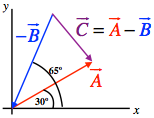
The angle between \(\overrightarrow A\) and \(\overrightarrow B\) is obviously 65º – 30º = 35º, so for this triangle we have the lengths of two sides and the angle between them. We can therefore find the length of the third side (\(\overrightarrow C\)) from the law of cosines:

\[{C^2} = {A^2} + {B^2} - 2AB\cos \theta \;\;\; \Rightarrow \;\;\;C = \sqrt {{{\left( {132} \right)}^2} + {{\left( {145} \right)}^2} - 2\left( {132} \right)\left( {145} \right)\cos \left( {{{35}^o}} \right)} = 84.2\nonumber\]

Next we can determine the angle between \(\overrightarrow A\) and \(\overrightarrow C\) using the law of sines:

\[\frac{\sin {35}^o}{C} = \frac{\sin \theta _{AC}}{B}\;\;\; \Rightarrow \;\;\;\theta _{AC} = \sin ^{ - 1}\left[ \frac{145}{84.2}\sin {35}^o \right] = 81^o\nonumber\]

If we rotate \(\overrightarrow C\) counterclockwise through this angle, it will be parallel to \(\overrightarrow A\), if we then rotated it back clockwise by 30º (the angle \(\overrightarrow A\) makes with the \(x\)-axis), then it will be parallel to the \(x\)-axis. Therefore the angle \(\overrightarrow C\) makes with the \(x\)-axis is: –81º + 30º = –51º (below the \(x\)-axis). This answer certainly conforms with the diagram above, which shows \(\overrightarrow C\) with a smaller magnitude than \(\overrightarrow A\) and \(\overrightarrow B\) and pointing down to the right.

While we can use these tools to mathematically solve for the sum of two vectors, it turns out that there is another way we can do it that doesn’t require quite as much geometrical reasoning. This method exploits three simple facts:

• We can replace any single vector as a sum of two (or more) vectors.
• It is easy to add two vectors that are parallel.
• If we use right triangles, trigonometry is easier to work with than with general triangles and the law of cosines/sines.

The trick is to select two (or three, if necessary) perpendicular axes (they do not have to be horizontal and vertical, they only need to be perpendicular to each other), and break up every vector involved into a sum of two perpendicular vectors parallel to these axes. The lengths of these perpendicular vectors are called the components of the vector along those axes. Going back to the list of advantages above, remember that we can add similar components like numbers, and we can determine these components easily using trigonometry.

Figure 1.1.3 – Vector Components

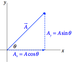
Figure 1.1.4 – Summing Vectors Using Components

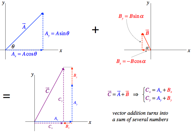
The sums of components are like summing numbers, but only components along the same axes can be added. The results are then more components, which then have to be reconstructed into a vector.

Unit Vectors

So we can use perpendicular coordinate systems to describe vectors in terms of their components. Essentially this means that to describe a vector in terms of a set of three axes, we need to know three numbers. But it might be useful to actually express these vectors as a single mathematical entity, and that’s where the notion of the unit vector comes in. Vectors have magnitude and direction, and with unit vectors we can mathematically break up the vector into those two parts. The magnitude is just a number (with physical units) without direction, and a unit vector is a vector (without units) that has a length of 1, so that it can be scaled to any length without contributing anything to the magnitude. Therefore we can write a vector as a simple product:

\[\overrightarrow A = A\widehat A\]

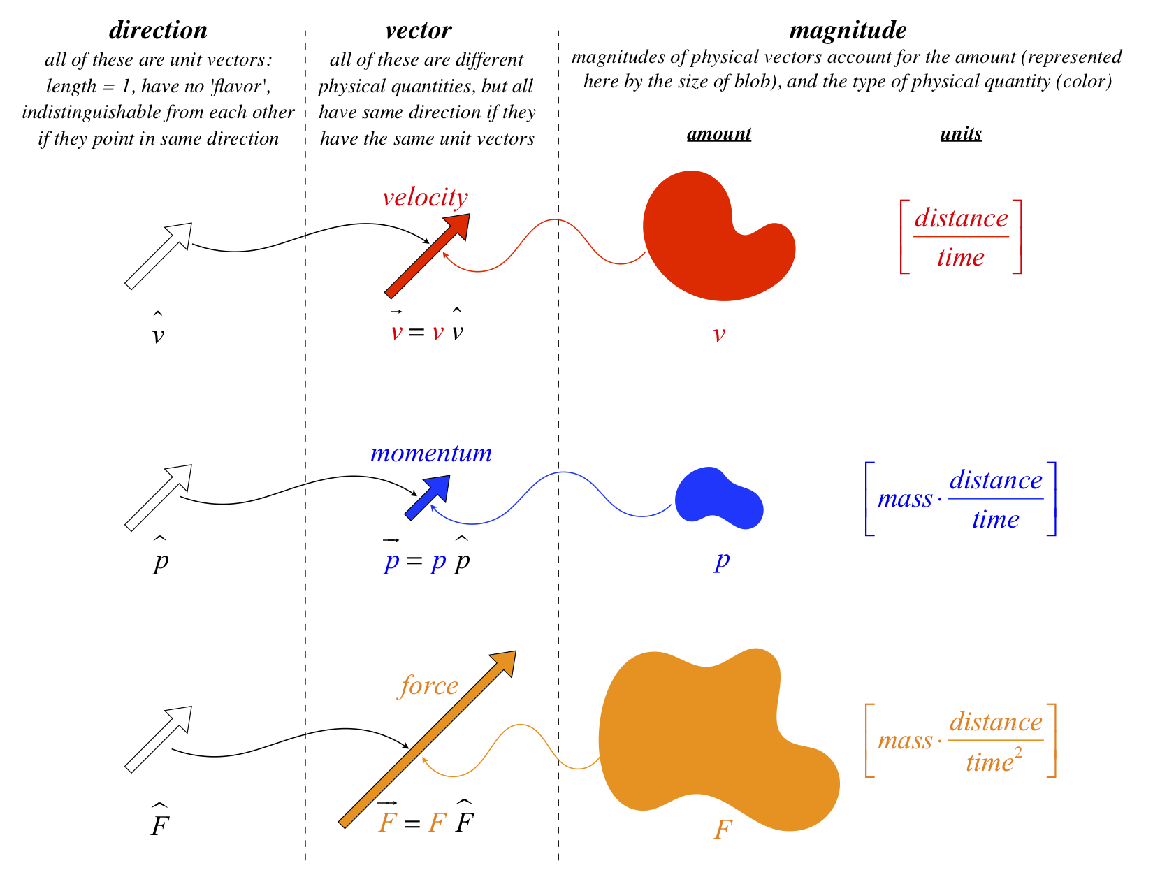
where \(\widehat A\) is the unit vector (usually pronounced “\(A\)-hat”). It is a unitless vector of length 1 that points in the direction of the vector \( \overrightarrow A\). The value \(A\) is a number with physical units that equals the magnitude. The diagram below gives a graphic description of how this construction works for a few common physical vectors. The unit vectors provide a very basic template by defining the direction, and the magnitude fills in the template by contributing the girth and 'flavor' (physical units) of the vector.

Figure 1.1.4 – Unit Vectors and Magnitudes

If we combine this notion with components, we can write any vector as a sum of components multiplying unit vectors in the directions of the three spatial dimensions. By convention, we give these unit vectors the names \(\widehat i\), \(\widehat j\), and \(\widehat k\) for the axes \(x\), \(y\), and \(z\), respectively. So specifically, we have:

\[\overrightarrow A = A_x\widehat i + A_y\widehat j + A_z\widehat k \]

Now we can just use this as a mathematical representation of vectors, and we do not have to appeal to geometry at all. For example,

\[ \begin{align} \overrightarrow C &= \overrightarrow A + \overrightarrow B \nonumber\\[5pt] &= (A_x\widehat i + A_y\widehat j + A_z\widehat k) + (B_x\widehat i + B_y\widehat j + B_z\widehat k) \nonumber\\[5pt] &= C_x\widehat i + C_y\widehat j + C_z\widehat k\nonumber\\[5pt] &= (A_x+ B_x) \widehat i + (A_y + B_y) \widehat j + (A_z + B_z) \widehat k \end{align}\]

Giving us the same result as we got before for the components of the sum of two vectors.

Exercise

Repeat the calculation of the previous Exercise, this time using components.

Solution

Breaking the two vectors into their \(x\) and \(y\) components gives:

\[\begin{array}{c} \overrightarrow A = {A_x}\widehat i + {A_y}\widehat j = A\cos \theta \;\widehat i + A\sin \theta \;\widehat j = 132\cos {30^o}\widehat i + 132\sin {30^o}\widehat j = 114.3\;\widehat i + 66.0\;\widehat j\\ \overrightarrow B = {A_x}\widehat i + {A_y}\widehat j = B\cos \theta \;\widehat i + B\sin \theta \;\widehat j = 145\cos {65^o}\widehat i + 145\sin {65^o}\widehat j = 61.3\;\widehat i + 131.4\;\widehat j \end{array}\nonumber\]

Next we subtract \(\overrightarrow B\) from \(\overrightarrow A\) to get \(\overrightarrow C\), then compute its magnitude (using the Pythagorean theorem) and direction (using trigonometry):

\[\begin{array}{l} \overrightarrow C = \overrightarrow A - \overrightarrow B = 53.0\;\widehat i - 65.4\;\widehat j\\ \left| {\overrightarrow C } \right| = \sqrt {{53.0}^2 + {65.4}^2} = 84.2\\ angle = \tan ^{ - 1}\left( \dfrac{ - 65.4}{53.0} \right) = - {51^o} \end{array}\nonumber\]

This matches the answer found in in the previous exercise.