6.2: Particle-in-a-Box, Part 2

The Time-Dependent Stationary-State Wave Functions

It's tempting to think that everything about the infinite square well was solved in the previous section, but that was only the stationary states! Remember that there are infinitely-more solutions that can be built from those. A good starting point is to have a visual model for what is going on with these energy eigenstates. Even though we solved for the time-independent wave function \(\psi\left(x\right)\), the full wave function for he quantum state of one of these energy eigenstates still has a time component to it:

\[\Psi_n\left(x,t\right)=\psi_n\left(x\right)e^{-i\omega_n t}=\sqrt{\frac{2}{L}}\sin\left(\frac{n\pi x}{L}\right)e^{-i\frac{E_n}{\hbar} t}~,~~~E_n=\frac{n^2h^2}{8mL^2}\]

We said that this is very similar to the solution of a standing wave on a string, and here we can see that the only difference is that it has both a real and imaginary sinusoid part to the time portion, while a standing wave on a string has only a real sinusoid for the time portion. So rather than having a mental picture of a string vibrating up-and-down, a better one is to think of a rotating jump-rope, with the antinodes swinging through the real and imaginary axes:

Figure 6.2.1 – Two Energy Eigenstates in a Box

These whirling jump-ropes represent the ground state and first-excited states of a particle in the infinite square well. There is one antinode for the ground state, and two for the first excited state, but the "oscillations" are not like those of a string standing wave. The figure defines "out of the page" as the positive imaginary axis, and "up" as the positive real axis (left-right is still the position (\(x\)) axis, with the left surface being \(x=0\) and the right \(x=L\)). Making this definition of the complex plane allows us to express the the time-dependent quantum phase as a rotation:

\[e^{-i\omega t}=\cos\omega t - i\sin\omega t\]

Notice that since \(\omega_n\propto E_n\propto n^2\), the \(n=2\) state has 4 times the rotational velocity as the \(n=1\) state.

Given the obvious time-dependence of these solutions, the question arise of why they are called stationary states. It's important to keep in mind that it is only the probability density that comes into the calculation our measurements, not the probability amplitude. The magnitude of the wave function is represented in the figure above by the distance that the "jump-rope" is from the straight line joining the endpoints. Because the jump-rope is rotating, any given point (measured by \(x\)) on it is always the same distance from the center line, which means that the probability amplitude magnitude remains fixed in time at any given position \(x\). With the probabilities of locating the particle at any position not changing, the state is indeed "stationary".

Non-Stationary-State Solutions

One might ask, "If the individual energy eigenstates are stationary, then why isn't a linear combination of them also stationary?" The answer lies once again in the figure above.  While each pieces of a single jump rope maintains a constant distance between it and the center line, if we add (like vectors) the position of two jump ropes representing different energies (attached at the same endpoints), then the fact they rotate at different speeds will mean that the net displacement changes with time. For example, the \(n=2\) eigenstate rotates at 4 times the rate of the \(n=1\) state, so one-half period for \(\Psi_1\) corresponds to two full periods for \(\Psi_2\). This means that if the antinode of \(\Psi_1\) is aligned in the same direction as the left antinode of \(\Psi_2\) at some initial time, then one-half period for \(\Psi_1\) later, its antinode will have flipped, while \(\Psi_2\) returns to its initial state since two of its full periods elapse.

Figure 6.2.2 – Superposed Eigenstates at Two Times

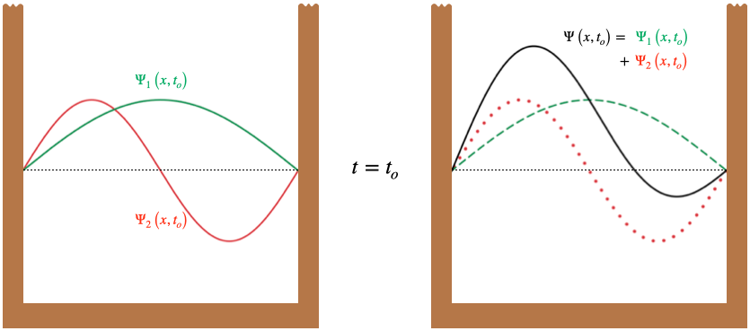
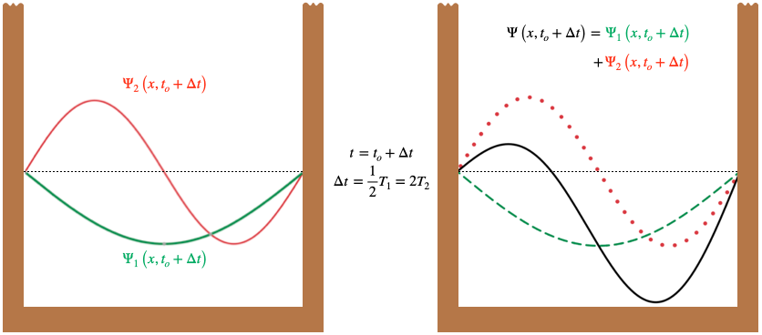
When the two wave functions superpose at these two times, the amplitude is larger in the left side of the box initially, and then larger in the right side of the box later. When this amplitude is squared to get the probability density, we find that the particle is more likely to be found in the left half of the box at the initial time, and more likely to be found in the right half of the box afterward – certainly the probability is not "stationary" in this case!

We will now invoke the spectral theorem to write the general solution of the Schrödinger equation. This consists of a linear combination of the energy eigenstates, with coefficients that define the "recipe" of that general state:

\[\Psi\left(x,t\right)=\sum\limits_{n=1}^\infty C_n\psi_n\left(x\right)e^{-i\omega_n t}=\sqrt{\frac{2}{L}}\sum\limits_{n=1}^\infty C_n\sin\left(\frac{n\pi x}{L}\right)e^{-i\frac{E_n}{\hbar} t}\]

If we look at the wave form of \(\Psi\) at \(t=0\), we see a very familiar sum: It is a Fourier series! We know exactly how to calculate the coefficients in this case – we use the orthogonality property of the eigenstates, namely:

\[C_n=\int\limits_0^L\psi^*_n\left(x\right)\Psi\left(x,0\right)dx\]

If the full wave function is known at some moment in time, then we can compute the entire eigenstate recipe (all of the \(C_n\)'s) of that state. Once all of these are known, the expectation value of the energy for \(\Psi\) can be computed using Equation 5.4.8. Note that the resulting state must still have the properties of a wave function that satisfies the Schrödinger equation for this potential (i.e. it must vanish at the walls), and it must be normalized. The first of these requirements is automatically satisfied, since every term in the sum has this property, and the second is a restriction on the coefficients, as we have already noted in Equation 5.4.7.

Emission and Absorption

Ultimately we hope that models like the infinite square well will help us to explain the world around us. It's pretty rare that one-dimensional models will give us directly usable results, but they are nevertheless useful for gaining insight into what comes later. When it comes to the "real world," experiments need to be performed to determine (or confirm) energy spectra like the one we found for this boxed particle. How exactly do we do this? Well, what we observe is virtually always light. We trust the principle of conservation of energy, and a particle that is trapped in a box can presumably absorb or emit light if the change in its energy level is equal to the energy of the photon it absorbs or emits (obviously an absorption results in an increase of energy level, and an emission a decrease). The frequency of the photon is then:

\[hf=\Delta E=E_{n_2}-E_{n_1}~~~\Rightarrow~~~f=\frac{1}{h}\left(\frac{h^2n_2^2}{8mL^2}-\frac{h^2n_1^2}{8mL^2}\right)=\frac{h}{8mL^2}\left(n_2^2-n_1^2\right)\]

The fact that the energy spectrum of the particle is quantized (the \(n\)'s are integers) means that the spectrum of the light emitted by the particle comes only in discrete frequencies. Every model will have its own particular spectrum. This particular model has energy levels proportional to \(n^2\), but we will see others during our journey, and the rough features of this spectrum are predictable based on certain qualities of the potential energy function.