
6.1: Atomic force microscopy (AFM) on Membranes
- Page ID
- 875
\( \newcommand{\vecs}[1]{\overset { \scriptstyle \rightharpoonup} {\mathbf{#1}} } \)
\( \newcommand{\vecd}[1]{\overset{-\!-\!\rightharpoonup}{\vphantom{a}\smash {#1}}} \)
\( \newcommand{\dsum}{\displaystyle\sum\limits} \)
\( \newcommand{\dint}{\displaystyle\int\limits} \)
\( \newcommand{\dlim}{\displaystyle\lim\limits} \)
\( \newcommand{\id}{\mathrm{id}}\) \( \newcommand{\Span}{\mathrm{span}}\)
( \newcommand{\kernel}{\mathrm{null}\,}\) \( \newcommand{\range}{\mathrm{range}\,}\)
\( \newcommand{\RealPart}{\mathrm{Re}}\) \( \newcommand{\ImaginaryPart}{\mathrm{Im}}\)
\( \newcommand{\Argument}{\mathrm{Arg}}\) \( \newcommand{\norm}[1]{\| #1 \|}\)
\( \newcommand{\inner}[2]{\langle #1, #2 \rangle}\)
\( \newcommand{\Span}{\mathrm{span}}\)
\( \newcommand{\id}{\mathrm{id}}\)
\( \newcommand{\Span}{\mathrm{span}}\)
\( \newcommand{\kernel}{\mathrm{null}\,}\)
\( \newcommand{\range}{\mathrm{range}\,}\)
\( \newcommand{\RealPart}{\mathrm{Re}}\)
\( \newcommand{\ImaginaryPart}{\mathrm{Im}}\)
\( \newcommand{\Argument}{\mathrm{Arg}}\)
\( \newcommand{\norm}[1]{\| #1 \|}\)
\( \newcommand{\inner}[2]{\langle #1, #2 \rangle}\)
\( \newcommand{\Span}{\mathrm{span}}\) \( \newcommand{\AA}{\unicode[.8,0]{x212B}}\)
\( \newcommand{\vectorA}[1]{\vec{#1}} % arrow\)
\( \newcommand{\vectorAt}[1]{\vec{\text{#1}}} % arrow\)
\( \newcommand{\vectorB}[1]{\overset { \scriptstyle \rightharpoonup} {\mathbf{#1}} } \)
\( \newcommand{\vectorC}[1]{\textbf{#1}} \)
\( \newcommand{\vectorD}[1]{\overrightarrow{#1}} \)
\( \newcommand{\vectorDt}[1]{\overrightarrow{\text{#1}}} \)
\( \newcommand{\vectE}[1]{\overset{-\!-\!\rightharpoonup}{\vphantom{a}\smash{\mathbf {#1}}}} \)
\( \newcommand{\vecs}[1]{\overset { \scriptstyle \rightharpoonup} {\mathbf{#1}} } \)
\(\newcommand{\longvect}{\overrightarrow}\)
\( \newcommand{\vecd}[1]{\overset{-\!-\!\rightharpoonup}{\vphantom{a}\smash {#1}}} \)
\(\newcommand{\avec}{\mathbf a}\) \(\newcommand{\bvec}{\mathbf b}\) \(\newcommand{\cvec}{\mathbf c}\) \(\newcommand{\dvec}{\mathbf d}\) \(\newcommand{\dtil}{\widetilde{\mathbf d}}\) \(\newcommand{\evec}{\mathbf e}\) \(\newcommand{\fvec}{\mathbf f}\) \(\newcommand{\nvec}{\mathbf n}\) \(\newcommand{\pvec}{\mathbf p}\) \(\newcommand{\qvec}{\mathbf q}\) \(\newcommand{\svec}{\mathbf s}\) \(\newcommand{\tvec}{\mathbf t}\) \(\newcommand{\uvec}{\mathbf u}\) \(\newcommand{\vvec}{\mathbf v}\) \(\newcommand{\wvec}{\mathbf w}\) \(\newcommand{\xvec}{\mathbf x}\) \(\newcommand{\yvec}{\mathbf y}\) \(\newcommand{\zvec}{\mathbf z}\) \(\newcommand{\rvec}{\mathbf r}\) \(\newcommand{\mvec}{\mathbf m}\) \(\newcommand{\zerovec}{\mathbf 0}\) \(\newcommand{\onevec}{\mathbf 1}\) \(\newcommand{\real}{\mathbb R}\) \(\newcommand{\twovec}[2]{\left[\begin{array}{r}#1 \\ #2 \end{array}\right]}\) \(\newcommand{\ctwovec}[2]{\left[\begin{array}{c}#1 \\ #2 \end{array}\right]}\) \(\newcommand{\threevec}[3]{\left[\begin{array}{r}#1 \\ #2 \\ #3 \end{array}\right]}\) \(\newcommand{\cthreevec}[3]{\left[\begin{array}{c}#1 \\ #2 \\ #3 \end{array}\right]}\) \(\newcommand{\fourvec}[4]{\left[\begin{array}{r}#1 \\ #2 \\ #3 \\ #4 \end{array}\right]}\) \(\newcommand{\cfourvec}[4]{\left[\begin{array}{c}#1 \\ #2 \\ #3 \\ #4 \end{array}\right]}\) \(\newcommand{\fivevec}[5]{\left[\begin{array}{r}#1 \\ #2 \\ #3 \\ #4 \\ #5 \\ \end{array}\right]}\) \(\newcommand{\cfivevec}[5]{\left[\begin{array}{c}#1 \\ #2 \\ #3 \\ #4 \\ #5 \\ \end{array}\right]}\) \(\newcommand{\mattwo}[4]{\left[\begin{array}{rr}#1 \amp #2 \\ #3 \amp #4 \\ \end{array}\right]}\) \(\newcommand{\laspan}[1]{\text{Span}\{#1\}}\) \(\newcommand{\bcal}{\cal B}\) \(\newcommand{\ccal}{\cal C}\) \(\newcommand{\scal}{\cal S}\) \(\newcommand{\wcal}{\cal W}\) \(\newcommand{\ecal}{\cal E}\) \(\newcommand{\coords}[2]{\left\{#1\right\}_{#2}}\) \(\newcommand{\gray}[1]{\color{gray}{#1}}\) \(\newcommand{\lgray}[1]{\color{lightgray}{#1}}\) \(\newcommand{\rank}{\operatorname{rank}}\) \(\newcommand{\row}{\text{Row}}\) \(\newcommand{\col}{\text{Col}}\) \(\renewcommand{\row}{\text{Row}}\) \(\newcommand{\nul}{\text{Nul}}\) \(\newcommand{\var}{\text{Var}}\) \(\newcommand{\corr}{\text{corr}}\) \(\newcommand{\len}[1]{\left|#1\right|}\) \(\newcommand{\bbar}{\overline{\bvec}}\) \(\newcommand{\bhat}{\widehat{\bvec}}\) \(\newcommand{\bperp}{\bvec^\perp}\) \(\newcommand{\xhat}{\widehat{\xvec}}\) \(\newcommand{\vhat}{\widehat{\vvec}}\) \(\newcommand{\uhat}{\widehat{\uvec}}\) \(\newcommand{\what}{\widehat{\wvec}}\) \(\newcommand{\Sighat}{\widehat{\Sigma}}\) \(\newcommand{\lt}{<}\) \(\newcommand{\gt}{>}\) \(\newcommand{\amp}{&}\) \(\definecolor{fillinmathshade}{gray}{0.9}\)Atomic force microscopy (AFM) is a technique with multiple applications in biology. This method is a member of the broad family of scanning probe microscopy and was initially developed in 1986 by Binnig et al to overcome the disadvantages of the scanning tunneling microscopy (STM) [1]. In the case of STM, only conductive materials can be studied as the resolution is obtained by using a tunneling current between a sharp probe and the sample surface[1]. In contrast, AFM uses small forces on the surface by a probe, thus do not damage samples and can provide information of surface topography of biological materials. AFM soon attracted the attention of the biophysical scientists in biomembrane as well as synthetic membrane research due to its capability of observing biological molecular system with resolution on nanometer scale and its possibility of three dimensional imaging [2].
Fundamental Elements of AFM
An atomic force microscope consists of a flexible cantilever containing a sharp probe, laser, photodiode detector, piezoelectric scanner and feedback electronics [3]. The microscope obtains the surface topography by scanning the tip in gentle touch with the sample. The tip motion is monitored by the piezoelectric scanner. As the tip scans the sample, the forces between the tip and the sample surface cause the cantilever to bend. A photodiode detector detects the deflection of a laser beam reflected off the back of the cantilever onto a two- segment photodiode. In most operating modes, a feedback circuit connected to the cantilever deflection sensor keeps the interaction between the tip and the sample at a fixed value and controls the tip-sample distance. The feedback signal is recorded by a computer to reconstruct a 3D image of the surface topography.

The force between the probe and the sample surface depends on the spring constant (stiffness of the cantilever) and the tip-sample distance). The amount of force is calculated based on Hooke’s law:
\[F= - kx\]
- \(F\): Force
- \(k\): spring constant
- \(x\): cantilever deflection.
Imaging modes
There are three primary imaging modes in AFM: contact, non-contact and intermittent (tapping) mode [4]. During contact mode, the probe is in contact with the sample and repulsive Van der Waals forces prevail, whilst attractive Van der Waals forces are dominant when the tip moves further away from the sample surface [5].

Contact Mode
In contact mode, the tip is constantly in touch with the sample surface. The applied force is kept constant while the tip scans the surface, creating the surface image [4]. This imaging mode is good for samples with rough and rigid surfaces as it provides fast scanning with high resolution. One disadvantage of this imaging mode is that soft samples like tissues can be deformed or damaged due to the applied force. This drawback can be solved by measuring the sample in aqueous environments to reduce the interaction force between the tip and the sample.
Tapping Mode
In tapping mode, the tip is not in constant contact with the sample surface. Instead, the cantilever is oscillated at its resonant frequency, which makes the tip lightly tap on the surface during scanning. A constant tip-sample interaction is maintained by monitoring the oscillation amplitude and an image is obtained [4]. Several parameters that affect the image contrast are the height, phase signals and amplitude [6]. Phase signals are influenced by material properties of the sample, for example viscoelasticity [6]. The force during scanning is greatly reduced, therefore this mode is useful for biological samples, where the samples are easily damageable or loosely bound to their surface. However, this imaging mode requires a slower scanning speed and is more challenging to measure in liquids.

Non-contact mode
There is no contact between the sample surface and the probe in non-contact mode. The probe oscillates above the sample surface, forming a weak attractive force between the tip apex atom and the sample surface atom. Feedback signals are obtained by measuring a frequency shift in the mechanical oscillation of the cantilever [6].
The force exerted on the surface sample is very low in this case. Moreover, as there is no contact between the probe and the surface, the probe lifetime can be extended. Another advantage of this operating mode is the possibility to observe an atomic defect if the very weak attractive force can be detected. The drawback of this mode is the reduction of resolution, and the oscillation of the cantilever is affected in case there are contaminants on the sample surface. Usually this operation mode requires a careful control of the environment (in UHV) to carry out [7].
Cantilever and Tips
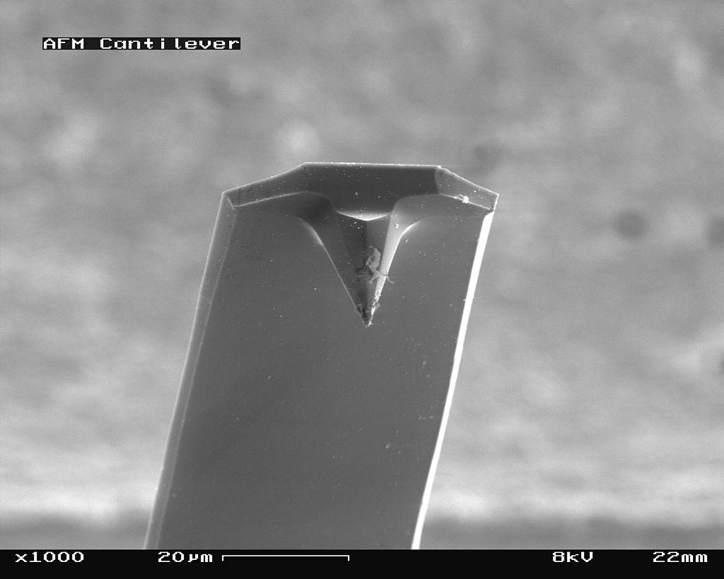
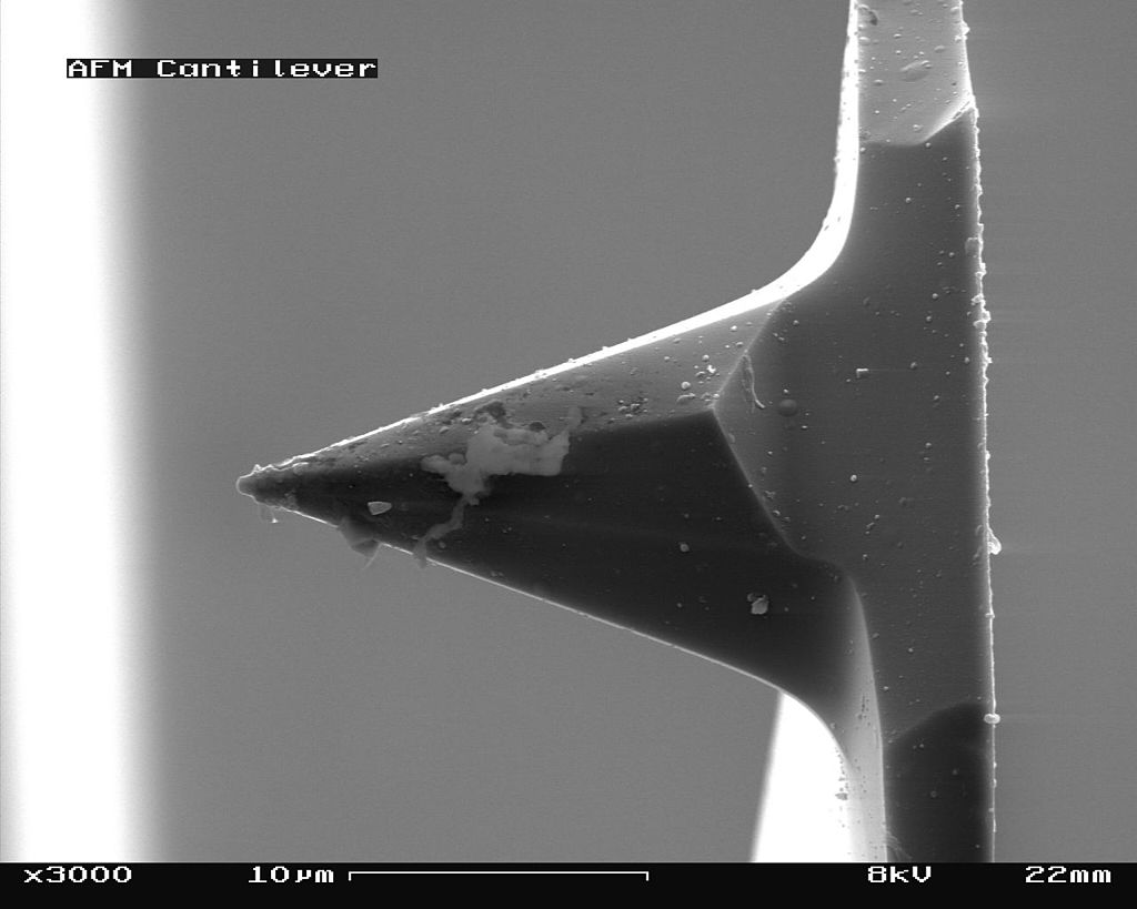
The scanning probe is an important component of the AFM. The dimensions of the cantilever are in micrometer range, while its tip has a radius of a few nanometers [4]. Different cantilever lengths, shapes and materials lead to various spring constants and resonant frequencies. The most common materials of the probes are silicon nitride (Si3N4) or silicon (Si) [5]. Figure \(\PageIndex{4}\) shows a scanning electron microscope (SEM) image of a silicon nitride (4a, 4b) and silicon (4c, 4d) cantilever chip, where a tiny tip having a pyramid shape is integrated at the end. The silicon nitride probe is often used in static contact mode, where the stiffness of the cantilever should be as low as possible [4]. The silicon probe is usually used in dynamic operation mode, which requires higher values for the spring constant to reduce noise and instabilities [4].
_cantilever_in_Scanning_Electron_Microscope%252C_magnification_1000x.jpg?revision=1&size=bestfit&width=375&height=300)
_cantilever_in_Scanning_Electron_Microscope%252C_magnification_3000x.jpg?revision=1&size=bestfit&width=375&height=300)
Typically, spring constants of AFM cantilevers vary between 0.01 Nm-1 and 100 Nm-1, enabling a force sensitivity of 10-11N [4]. The force sensitivity is influenced by thermal, electrical and optical noise. [5] For biological samples, cantilevers in contact mode often have resonance frequencies between 5 and 50 kHz in vacuum [8]. Figure \(\PageIndex{5}\) reports an AFM tip made of carbon nanotubes (CNTs), which was a breakthrough in terms of resolution. CNTs tips have a high aspect ratio, small diameter, and a well-defined surface chemistry, therefore appearing to be the ideal probe for biological applications [4].

AFM on membranes
Native membranes studied by AFM
Biomembrane sample preparation
In order to study membranes using AFM, the membranes need to be fixed on a flat solid support [8]. Several solid supports such as mica, highly ordered pyrolitic graphite (HOPG), template stripped gold and molybdenum disulfide have proved to give high resolution images [6, 8]. While mica is an insulator and exposes a hydrophilic surface, HOPG is a good conductor and hydrophobic [8]. The similarity between these two substrates is an atomically flat surface [8]. Based on chemical adsorption mechanism, membranes are attached onto the solid support by adjusting pH and ionic strength. As the gap between membrane and the support is very small (0.5-2nm), this may cause impaired mobility for membrane proteins that are directly attached to the support [6]. Furthermore, the adsorption force may affect the conformation of the membrane proteins. To sum up, current sample preparation methods still need further consideration in order to study dynamics and structure of native membrane proteins.
AFM images of native membrane
AFM can obtain the images of native membranes at submolecular resolution, which is a great advantage comparing to other methods [6]. It is effective in providing information of the native organization of membrane proteins and their complexes. Figure \(\PageIndex{6}\) shows an example of the study of native membrane using AFM. Disk membranes were prepared from mouse retina and then attached on mica support [6]. The AFM image revealed tight rows of dimers packed in the structure arrangement of rhodopsin [6]. This provides a platform for interaction with arrestin and transducin.

Model lipid membranes studied by AFM
Preparation of supported lipid bilayers.
Supported lipid bilayers (SLBs) have been used as a biomimetic model for biomembranes in numerous studies [3, 9]. This system consists of two lipid leaflets spread on a solid support [3]. Although this model lacks some features of the real membranes, it still provides an insight of the structural organization and characteristics of cell membranes. The first method to prepare SLBs is the fusion of lipid vesicles on solid supports [9]. The vesicles are prepared via sonication or extrusion, then adsorbed on the surface of the solid support. The adsorbed vesicles either form larger vesicles by fusing together, or directly rupture and form SLBs.
Another method is to use a hydrophilic substrate on which two consecutive lipid monolayers are deposited by Langmuir-Blodgett transfer [3]. A Teflon-coated trough contains the aqueous solution, with two movable Teflon barriers used to control the area for lipid spread and form a monolayer at the air-water interface. There is also a balance to measure the surface pressure, controlling lipid packing. The solid support is then pulled vertically through the lipid monolayer, depositing the first lipid layer on the substrate. The transference of the second lipid layer can be completed by dipping the lipid support either horizontally or vertically. This technique can be applied to fabricate SLBs having two different lipid composition.
AFM studies of SLBs formation.
SLBs formation process by fusing lipid vesicles on solid supports can be studied in situ by AFM technique, as illustrated in Figure \(\PageIndex{7}\). The vesicles spread from the edge towards the center, then stacked on top of each other. The edges of the top and bottom bilayers are joined together to form bigger patches.

Different protocols to prepare multi-component and phase-separated SLBs can affect the asymmetry of the resulting SLBs. In Figure \(\PageIndex{8}\), the extruded small unilamellar vesicles (SUVs) composed of DLPC/DSPC are heated at 650C, then fused on mica at 200C. The resulting SLB are fully symmetric fluid/gel membranes. On the other hand, using sonicated SUVs heated at 200C prior to fusion results in a completely asymmetric SLBs.

Summary
AFM is a powerful technique for scientists to have an insight in membrane biophysics. Advantages of this method including:
- The ability to image cell surfaces, molecular assemblies in their native aqueous environment at a very high resolution.
- No requirement of a conductive sample.
- Provide 3-D surface profiles.
- The ability to operate in liquid environment and ambient air.
Disadvantages of AFM are limited scanning area and the scanning speed.
Recently there have been some progress in improving AFM scanning speed and resolution, for example high speed AFM (HS-AFM) or high resolution AFM (HR-AFM) [10, 11]. HF-AFM consists of modified components in order to maximize scanning seed, for example soft small cantilevers having high resonance frequencies, high resonance frequency scanners and fast data acquisition devices [10]. AFM is also combined with several techniques such as fluorescence microscopy to acquire more efficient data [9]. The potential improvement of AFM will enhance the possibility to apply this technique in a wider range of biological fields.
References
- Binnig, G., C. F. Quate, and C. Gerber, Atomic force microscope. Phys. Rev. Lett, 1986(56): p. 930–933.
- D.J.Muller, Y.F.D., Atomic force microscopy as a multifunctional molecular toolbox in nanobiotechnology. Nat.Nanotechnol, 2008. 3: p. 261-269.
- Morandat, S., et al., Atomic force microscopy of model lipid membranes. Anal Bioanal Chem, 2013. 405(5): p. 1445-61.
- Alessandrini, A. and P. Facci, AFM: a versatile tool in biophysics. Measurement Science and Technology, 2005. 16(6): p. R65- R92.
- Bullen, R.A.W.a.H.A., Lecture notes: Introduction to Scanning Probe Microscopy
- Frederix, P.L., P.D. Bosshart, and A. Engel, Atomic force microscopy of biological membranes. Biophys J, 2009. 96(2): p. 329- 38.
- S. Morita, R.W., E. Meyer, Noncontact Atomic Force Microscopy. Springer, 2002. 1.
- Muller, D.J. and A. Engel, Atomic force microscopy and spectroscopy of native membrane proteins. Nat Protoc, 2007. 2(9): p. 2191-7.
- Goksu, E.I., et al., AFM for structure and dynamics of biomembranes. Biochim Biophys Acta, 2009. 1788(1): p. 254-66.
- Ando, T., T. Uchihashi, and N. Kodera, High-speed AFM and applications to biomolecular systems. Annu Rev Biophys, 2013. 42: p. 393-414.
- Bippes, C.A. and D.J. Muller, High-resolution atomic force microscopy and spectroscopy of native membrane proteins. Reports on Progress in Physics, 2011. 74(8): p. 086601.