7.3: Air Resistance Proportional to the Square of the Speed

Notation: $\bf V$ is the velocity, $V$ is the speed. The horizontal and vertical components of the velocity are, respectively, $u=\dot{x} = V \cos\psi$ and $v=\dot{y} = V sin\psi$. Here $\psi$ is the angle that the instantaneous velocity $\bf V$ makes with the horizontal. The resistive force per unit mass is $kV^{2}$. The horizontal and vertical components of the resistive force per unit mass are $kV^{2}cos\psi$ and $kV^{2}sin\psi$ respectively. The launch speed is $V_{0}$ and the launch angle (i.e. the initial value of $\psi$) is $\alpha$. Distance traveled from the launch point, measured along the trajectory, is $s$ and speed $V=\dot{s}$. The Equations of motion are:

Horizontal:

$$\ddot{x} = -kV^{2}\cos\psi \tag{7.3.1}\label{eq:7.3.1}$$

Vertical:

$$\ddot{y} = -g-kV^{2}\sin\psi \tag{7.3.2}\label{eq:7.3.2}$$

These cannot be integrated as conveniently as in the previous cases, but we can get a simple relation between the horizontal component $u$ of the speed and the intrinsic coordinate $s$. Thus, when we make use of $\ddot{x}=\dot{u}$, $V =\dot{s}$ and $Vcos\psi=u$, Equation $\ref{eq:7.3.1}$ takes the form

$$\dot{u} = -ku\dot{s} \tag{7.3.3}\label{eq:7.3.3}$$

Integration, with initial condition $u = V_{0}cos\theta$, yields

$$u=V_{0}\cos\alpha.e^{-ks}. \tag{7.3.4}\label{eq:7.3.4}$$

We can also obtain an exact explicit intrinsic Equation to the trajectory by consideration of the normal Equation of motion.

The intrinsic Equation to any curve is a relation between the intrinsic coordinates ($s$, $\psi$). The rate at which the slope angle $\psi$ changes as you move along the curve, i.e. $\frac{d\psi}{ds}$, is called the curvature at a point along the curve. If the slope is increasing with $s$, the curvature is positive. The reciprocal of the curvature at a point, $\frac{ds}{d\psi}$, is the radius of curvature at the point, denoted here by $\rho$.

The normal Equation of motion is the Equation $F = ma$ applied in a direction normal to the curve. The acceleration appropriate here is the centripetal acceleration $\frac{V^{2}}{\rho}$ or $V^{2}\frac{d\psi}{ds}$.

In a direction normal to the motion, the air resistance has no component, and gravity has a component $−g \cos\theta$. (It is minus because the curvature is clearly negative.) The normal Equation of motion is therefore

$$V^{2}\frac{d\psi}{ds}=−g \cos\theta. \tag{7.3.5}\label{eq:7.3.5}$$

But

$$V=\frac{u}{\cos\psi}=\frac{V_{0}\cos\alpha.e^{-ks}}{\cos\psi} \tag{7.3.6}\label{eq:7.3.6}$$

Therefore

$$V_{0}^{2}\cos^{2}\alpha.e^{-2ks}\frac{d\psi}{ds}=-g\cos^{3}\psi. \tag{7.3.7}\label{eq:7.3.7}$$

Separate the variables, and integrate, with appropriate initial conditions:

$$\int_{\alpha}^{\psi}\sec^{3}\psi d\psi=-\dfrac{g}{V_{0}^{2}\cos^{2}\alpha}\int_{0}^{s}e^{2ks}ds \tag{7.3.8}\label{eq:7.3.8}$$

From here it is good integration practice to show that the intrinsic Equation is

$$\sec\psi \tan\psi-\sec\alpha \tan\alpha+\ln \left(\frac{\sec\psi +\tan\psi}{\sec\alpha + \tan\alpha} \right) = \dfrac{g}{kV_{0}^{2}\cos^{2}\alpha}(1-e^{2ks}) \tag{7.3.9}\label{eq:7.3.9}$$

This Equation is of the form

$$\sec\psi \tan\psi + \ln \left(\sec\psi+\tan\psi \right) = A - Be^{2ks}. \tag{7.3.10}\label{eq:7.3.10}$$

While it would be straightforward now to compute $s$ as a function of $\psi$ and hence to plot a graph of $s$ versus $\psi$, we really want to show $y$ as a function of $x$, and $x$ and $y$ as a function of time. I am indebted to Dario Bruni of Italy for the following analysis.

Let ($x_{1}$ _, $y_{1}$) be a point on the trajectory. When the projectile moves a short distance $\Delta s$, the new coordinates will be ($x_{2}$_, $x_{2}$), where

$$x_{2}=x_{1}+\Delta s \cos\psi_{1} \tag{7.3.11}\label{eq:7.3.11}$$

and

$$y_{2}=y_{1}+\Delta s \sin\psi_{1}, \tag{7.3.12}\label{eq:7.3.12}$$

provided that $\Delta s$ is taken to be sufficiently small that the path between the two points is approximately a straight line. The calculation starts with $x_{1}$ = $y_{1}$ = 0 and $\psi$ = $\alpha$. At each stage of the calculation, the new value of $\psi$ can be calculated from Equation $\ref{eq:7.3.10}$. This can be done easily, for example, by Newton-Raphson iteration, since the derivative of the left hand side of this equation with respect to $\psi$ is just $2\sec^{3}\psi$. Thus, with a sufficiently small interval $\Delta s$, the shape of the trajectory can be built up point by point.

While this gives us the shape of the trajectory, it tells us nothing about the time. To do this, we can write the Equations of motion, Equations $\ref{eq:7.3.1}$ and $\ref{eq:7.3.2}$ in the forms

$$\ddot{x}=-k\dot{x}\sqrt{\dot{x}^{2}+\dot{y}^{2}} \tag{7.3.13}\label{eq:7.3.13}$$

and

$$\ddot{y}=-g-k\dot{y}\sqrt{\dot{x}^{2}+\dot{y}^{2}}. \tag{7.3.14}\label{eq:7.3.14}$$

Let ($x_{1}$ _, $y_{1}$) be a point on the trajectory. After a short time $\Delta t$, the new coordinates will be ($x_{2}$ _, $y_{2}$), where

$$x_{2}=x_{1}+\dot{x}_{1}\Delta t+\frac{1}{2}\ddot{x}_{1}(\Delta t)^{2} \tag{7.3.15}\label{eq:7.3.15}$$

and

$$y_{2}=y_{1}+\dot{y}_{1}\Delta t+\frac{1}{2}\ddot{y}_{1}(\Delta t)^{2}, \tag{7.3.16}\label{eq:7.3.16}$$

provided that $\Delta t$ is taken to be sufficiently small that the acceleration between the two instants of time is approximately constant. Also, the new velocity components are given by

$$\dot{x}_{2} = \dot{x}_{1} + \ddot{x}_{1}\Delta t \tag{7.3.17}\label{eq:7.3.17}$$

and

$$\dot{y}_{2} = \dot{y}_{1} + \ddot{y}_{1}\Delta t. \tag{7.3.18}\label{eq:7.3.18}$$

The calculation starts with

$\dot{x}=V_{0}\cos\alpha, \quad \dot{y}=V_{0}\sin\alpha, \quad \ddot{x}=-kV_{0}^{2}\cos\alpha, \quad \ddot{y}=-g-kV_{0}^{2}\sin\alpha$

and after each increment $\Delta t$ the new coordinates and velocity and acceleration components are calculated. The results of Sr Bruni’s calculations are shown in Figure VII.3 for

$k$ = 0.0177m^-1, $V_{0}$ = 90.5ms^-1, $\alpha$ = 60$^{\circ}$, $g$ = 9.8ms^-2

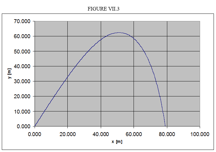
Plotted with step by step method from intrinsic Equation with $\Delta s$= 0.025 m. Horizontal range 79.0 m; maximum height 62.4 m. Total flight duration 7.1 seconds. The time taken to reach the maximum height is 2.8 seconds, so the descent time is longer than the ascent time.

An alternative approach has been given by Ambrose Okune, of Uganda. In Okune’s analysis, he obtains explicit expressions for $t$, $x$ and $y$in terms of the angle $\psi$. (In Equation $\ref{eq:7.3.10}$ we already have a relation between $s$ and $\psi$.)

We start with Equation $\ref{eq:7.3.1}$, the horizontal Equation of motion

$$\ddot{x} = -kV^{2}\cos\psi=-kVV\cos\psi. \tag{7.3.19}\label{eq:7.3.19}$$

Now $\ddot{x}=\dot{u}$, $V = \sqrt{u^{2}+v^{2}}$, and $V\cos\psi = u$ so that

$$\dot{u}=-ku\sqrt{u^{2}+v^{2}}. \tag{7.3.20}\label{eq:7.3.20}$$

Similarly, Equation $\ref{eq:7.3.2}$, the vertical Equation of motion, is

$$\ddot{y} = -g-kV^{2}\sin\psi = -g-kVV\sin\psi, \tag{7.3.21}\label{eq:7.3.21}$$

and, with $\ddot{y}=\dot{v}$, $V = \sqrt{u^{2}+v^{2}}$, and $V\sin\psi = v$,this becomes

$$\dot{v}=-g-kv\sqrt{u^{2}+v^{2}}. \tag{7.3.22}\label{eq:7.3.22}$$

Now

$$\frac{\dot{v}}{\dot{u}}=\frac{dv}{du}=\frac{v}{u}+\frac{g}{ku\sqrt{u^{2}+v^{2}}}. \tag{7.3.23}\label{eq:7.3.23}$$

Also $v$ = $u\tan\psi$ so that

$$\frac{dv}{du}=\tan\psi+usec^{2}\frac{d\psi}{du}. \tag{7.3.24}\label{eq:7.3.24}$$

On comparison of Equations $\ref{eq:7.3.23}$ and $\ref{eq:7.3.24}$, we see that

$$\frac{g}{ku\sqrt{u^{2}+v^{2}}}=u\sec^{3}\psi d\psi. \tag{7.3.25}\label{eq:7.3.25}$$

Upon substitution of $v$ = $u\tan\psi$ this becomes

$$\frac{g}{ku^{3}}=\sec^{3}\psi\frac{d\psi}{du}. \tag{7.3.26}\label{eq:7.3.26}$$

and hence

$$\frac{g}{k}\int_{}{}u^{-3}du=\int_{}{}\sec^{3}\psi d\psi. \tag{7.3.27}\label{eq:7.3.27}$$

Upon integration, we obtain

$$\frac{g}{ku^{2}}+\ln(\sec\psi+\tan\psi)+\sec\psi \tan\psi=A=\frac{g}{ku_{0}^{2}}+\ln(\sec\alpha+\tan\alpha)+\sec\alpha \tan\alpha. \tag{7.3.28}\label{eq:7.3.28}$$

From this, we obtain

$$u=\sqrt{\frac{g}{k}}\frac{1}{\sqrt{A-\ln(sec\psi+\tan\psi)-sec\psi \tan\psi}}, \tag{7.3.29}\label{eq:7.3.29}$$

and hence

$$v=\sqrt{\frac{g}{k}}\frac{\tan\psi}{\sqrt{A-\ln(sec\psi+tan\psi)-\sec\psi \tan\psi}}. \tag{7.3.30}\label{eq:7.3.30}$$

Thus we now have the velocity components explicitly in terms of the angle y. For simplicity, let us write

$$\lambda = A-\ln(\sec\psi+\tan\psi)-\sec\psi \tan\psi. \tag{7.3.31}\label{eq:7.3.31}$$

Then the Equations for the velocity components are

$$u=\sqrt{\frac{g}{k}}\frac{1}{\sqrt{\lambda}} \tag{7.3.32}\label{eq:7.3.32}$$

and

$$v=\sqrt{\frac{g}{k}}\frac{\tan\psi}{\sqrt{\lambda}}. \tag{7.3.33}\label{eq:7.3.33}$$

In the limit, as $u\rightarrow0$, $\psi\rightarrow-90^{\circ}$, $y\rightarrow-\infty$, the motion approaches a vertical asymptote. As $\psi\rightarrow-90^{\circ}$, $\lambda\rightarrow-sec\psi tan\psi$ and hence $\lim_{\psi\rightarrow-90^{\circ}}\frac{tan\psi}{\sqrt{\lambda}}=-1$. Thus the limiting value of the vertical component of the velocity is $-\sqrt{\frac{g}{k}}$. This agrees precisely with what one would expect for a body falling vertically at terminal speed, with resistance proportional to the square of the speed (see Equation 6.4.5).

We now aim to find an expression relating $\psi$ to $t$, which we do by noting that

$$\frac{d\psi}{dt}=\frac{\frac{du}{dt}}{\frac{du}{d\psi}}=\frac{\frac{du}{dt}}{\frac{du}{d\lambda}\frac{d\lambda}{d\psi}}. \tag{7.3.34}\label{eq:7.3.34}$$

The derivative $\frac{du}{dt}$ can be found from the horizontal Equation of motion $\ddot{x}=-kV^{2}cos\psi$, which can be written (because $u=V$ and $\ddot{x}=\dot{u}$) as $\dot{u}=-ku^{2}sec\psi$. Then, making use of Equation $\ref{eq:7.3.32}$, we obtain

$$\frac{du}{dt}=-\frac{g}{\lambda}\sec\psi \tag{7.3.35}\label{eq:7.3.35}$$

The derivative $\frac{du}{d\lambda}$ can be found from Equation $\ref{eq:7.3.32}$ and is

$$\frac{du}{d\lambda}=-\frac{1}{2}\sqrt{\frac{g}{k}}\frac{1}{\lambda^{\frac{3}{2}}}. \tag{7.3.36}\label{eq:7.3.36}$$

The derivative $\frac{d\lambda}{d\psi}$ can be found from Equation $\ref{eq:7.3.31}$ and is

$$\frac{d\lambda}{d\psi} = -2\sec^{3}\psi. \tag{7.3.37}\label{eq:7.3.37}$$

Thus the relation we seek is

$$\frac{d\psi}{dt} = -\sqrt{gk}\sqrt{\lambda}\cos^{2}\psi. \tag{7.3.38}\label{eq:7.3.38}$$

If the initial motion of the projectile at time zero makes an angle $\alpha$ with the horizontal, then integration of Equation $\ref{eq:7.3.38}$ gives the following expression for the subsequent time $t$ when the motion makes an angle $\psi$ with the horizontal.

$$t=\frac{1}{\sqrt{gk}}\int_{\psi}^{\alpha}\frac{d\psi}{\sqrt{\lambda}\cos^{2}\psi}. \tag{7.3.39}\label{eq:7.3.39}$$

Also $u$ = $\frac{dx}{dt}$ = $\frac{dx}{d\psi}$$\frac{d\psi}{dt}$. With $u$ and $\frac{d\psi}{dt}$ given respectively by Equations $\ref{eq:7.3.32}$ and $\ref{eq:7.3.38}$, we obtain

$$\frac{dx}{d\psi}=-\frac{1}{k\lambda \cos^{2}\psi}, \tag{7.3.40}\label{eq:7.3.40}$$

from which we can calculate $x$ as a function of $\psi$:

$$x = \frac{1}{k}\int_{\psi}^{\alpha}\frac{d\psi}{\lambda \cos^{2}\psi}. \tag{7.3.41}\label{eq:7.3.41}$$

Further, $v$ = $\frac{dy}{dt}$ = $\frac{dy}{d\psi}\frac{d\psi}{dt}$. With $v$ and $\frac{d\psi}{dt}$ given respectively by Equations $\ref{eq:7.3.33}$ and $\ref{eq:7.3.38}$, we obtain

$$\frac{dy}{d\psi}=-\frac{\tan\psi}{k\lambda \cos^{2}\psi}, \tag{7.3.42}\label{eq:7.3.42}$$

from which we can calculate $y$ as a function of $\psi$:

$$y =\frac{1}{k}\int_{\psi}^{\alpha}\frac{\tan\psi d\psi}{\lambda \cos^{2}\psi}. \tag{7.3.43}\label{eq:7.3.43}$$

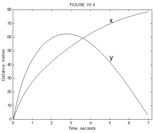
Equations $\ref{eq:7.3.39}$, $\ref{eq:7.3.41}$ and $\ref{eq:7.3.43}$ enable us to calculate $t$, $x$ and $y$ as a function of $\psi$, and hence to calculate any one of them in terms of any of the others. In each case a numerical integration is required, such as by Simpson’s rule or by Gaussian quadrature, or other integration algorithm, and, as is always the case, sufficient points must be sampled to obtain adequate precision. Numerical integration of these Equations, using the data of Dario Bruno’s example above, produced the same $x$ : $y$ trajectory as calculated for Figure VII.3 by Bruno, and the $x$ : $t$ and $y$ : $t$ relations shown in Figure VII.4.

I am greatly indebted to Dario Bruni and to Ambrose Okune for their interesting and instructive contributions to this section – an inspirational example of international scientific cooperation between, Italy, Uganda and Canada!