
11.4: Curve of Growth for Gaussian Profiles
- Page ID
- 6716

By “gaussian profile” in the title of this section, I mean profiles that are gaussian in the optically-thin case; as soon as there are departures from optical thinness, there are also departures from the gaussian profile. Alternatively, the absorption coefficient and the optical depth are gaussian; the absorptance is not.
For an optically-thin thermally-broadened line, the optical thickness as a function of wavelength is given by
\[\label{11.4.1}\tau (x)=\tau (0)\text{exp}\left ( -\frac{x^2\ln 2}{g^2}\right ) ,\]
where the HWHM is
\[\label{11.4.2}g=\frac{V_m \lambda_0 \sqrt{\ln 2}}{c}.\]
Here \(V_\text{m}\) is the modal speed. (See Chapter 10 for details.) The line profiles, as calculated from equations 11.3.4 and \ref{11.4.1}, are shown in figure XI.2 for the following values of the optical thickness at the line centre: \(\tau (0)=\frac{1}{16},\frac{1}{8},\frac{1}{4},\frac{1}{2},1,2,4,8.\)
On combining equations 11.3.4 and \ref{11.4.1} and \ref{11.4.2}, we obtain the following expression for the equivalent width:
\[\label{11.4.3}W=2\int_0^\infty \left ( 1-\text{exp}\left \{-\tau (0)e^{-x^2\ln 2/g^2}\right \}\right )\,dx,\]
or
\[\label{11.4.4}W=\frac{2V_\text{m}\lambda_0}{c}\int_0^\infty \left ( 1-\text{exp}\left \{-\tau(0)e^{-\Delta^2}\right \}\right )\,d\Delta,\]
where
\[\label{11.4.5}\Delta =\frac{x\sqrt{\ln 2}}{g}=\frac{cx}{V_\text{m}\lambda_0}.\]
The half-width at half maximum (HWHM) of the expression \ref{11.4.1} for the optical thickness corresponds to \(\Delta = \sqrt{\ln 2} = 0.8326\). For the purposes of practical numerical integration of Equation \ref{11.4.4}, I shall integrate from \(\Delta = -5\text{ to }+5\) that is to say from \(\pm 6\) times the HWHm. One can appreciate from figure XI.2 that going outside these limits will not contribute significantly to the equivalent width. I shall calculate the equivalent width for central optical depths ranging from \(1/20 (\log \tau (0) = −1.3)\text{ to }10^5 (\log \tau (0) = 5.0)\).
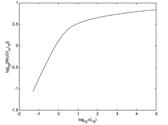
What we have in figure XI.3 is a curve of growth for thermally broadened lines (or lines that, in the optically thin limit, have a gaussian profile, which could include a thermal and a microturbulent component). I have plotted this from \(\log \tau(0) = -1.3\text{ to }+5.0\); that is \(\tau(0) = 0.05\text{ to }10^5\).
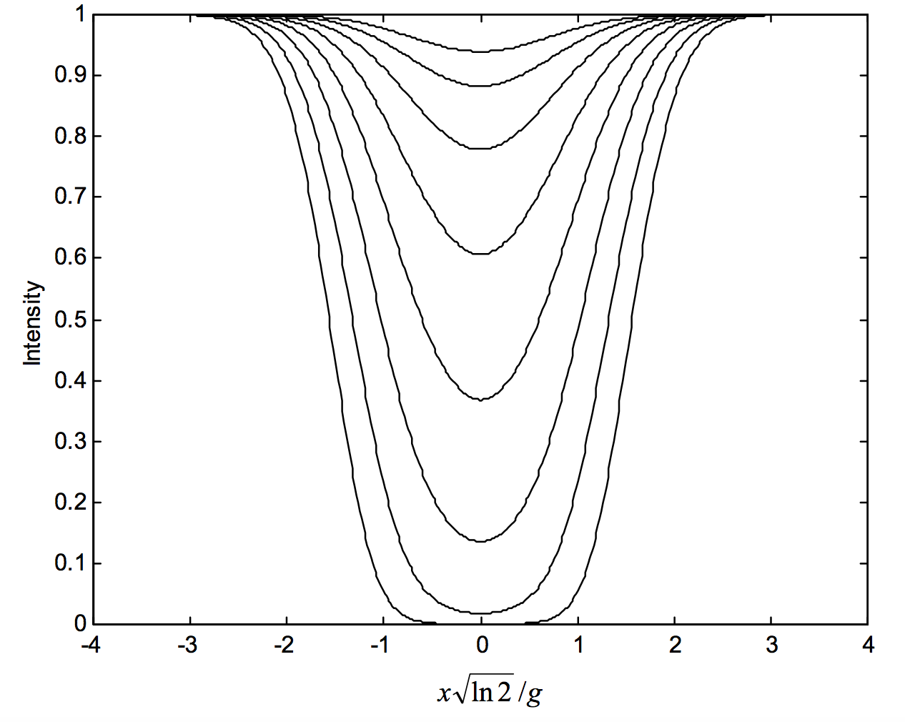
\(\text{FIGURE XI.2}\)
\(\text{FIGURE XI.3}\)