
B22: Huygens’s Principle and 2-Slit Interference


- Last updated
- Apr 24, 2022
- Save as PDF

( \newcommand{\kernel}{\mathrm{null}\,}\)
Consider a professor standing in front of the room holding one end of a piece of rope that extends, except for sag, horizontally away from her in what we’ll call the forward direction. She asks, “What causes sinusoidal waves?” You say, “Something oscillating.” “Correct,” she replies. Then she starts moving her hand up and down and, right before your eyes, waves appear in the rope. For purposes of discussion, we will consider the waves only before any of them reach the other end, so we are dealing with traveling waves, not standing waves. “What, specifically, is causing these waves,” she asks, while pointing, with her other hand, at the waves in the rope. You answer that it is her hand oscillating up and down that is causing the waves and again you are right. Now suppose you focus your attention on a point in the rope, call it point P, somewhat forward of her hand. Like all points in the rope where the wave is, that point is simply oscillating up and down. At points forward of point P, the rope is behaving just as if the professor were holding the rope at point P and moving her hand up and down the same way that point P is actually moving up and down. Someone studying only those parts of the rope forward of point P would have no way of knowing that the professor is actually holding onto the rope at a point further back and that point P is simply undergoing its part of the wave motion caused by the professors hand at the end of the rope. For points forward of point P, things are the same as if point P were the source of the waves. For predicting wave behavior forward of point P, we can treat point P, an oscillating bit of the rope, as if it were the source of the waves. This idea that you can treat one point in a wave medium as if it were the source of the waves forward of it, is called Huygens’s Principle. Here, we have discussed it in terms of a one dimensional medium, the rope. When we go to more than one dimension, we can do the same kind of thing, but we have more than one point in the wave medium contributing to the wave behavior at forward points. In the case of light, that which is oscillating are the electric field and the magnetic field. For smooth regular light waves traveling in a forward direction, if we know enough about the electric and magnetic fields at all points on some imaginary surface through which all the light is passing, we can determine what the light waves will be like forward of that surface by treating all points on the surface as if they were point sources of electromagnetic waves. For any point forward of the surface, we just have to (vectorially) add up all the contributions to the electric and magnetic fields at that one point, from all the “point sources” on the imaginary surface. In this chapter and the next, we use this Huygens’s Principle idea in a few simple cases (e.g. when, except for two points on the kind of surface just mentioned, all the light is blocked at the surface so you only have two “point sources” contributing to the electric and magnetic fields at points forward of the surface—you could create such a configuration by putting aluminum foil on the surface and poking two tiny holes in the aluminum foil) to arrive at some fairly general predictions (in equation form) regarding the behavior of light. The first has to do with a phenomenon called two-slit interference. In applying the Huygens’s principle idea to this case we use a surface that coincides with a wave front. In diagrams, we have some fairly abstract ways of representing wave fronts which we share with you by means of a series of diagrams of wave fronts, proceeding from less abstract to more abstract.
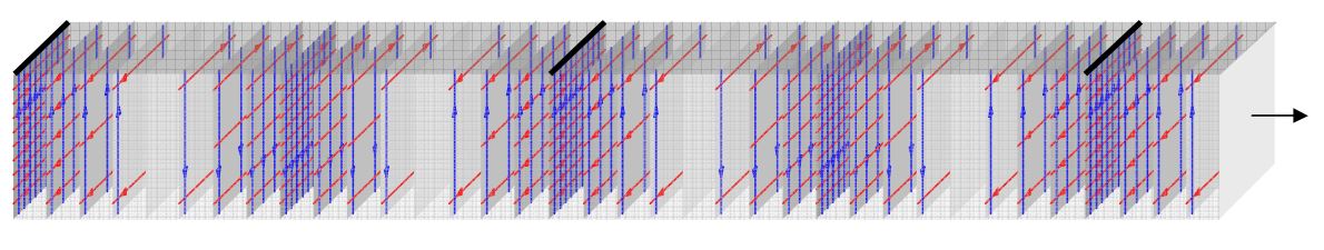
Here’s one way of depicting a portion of a beam of light traveling forward through space, at an instant in time:
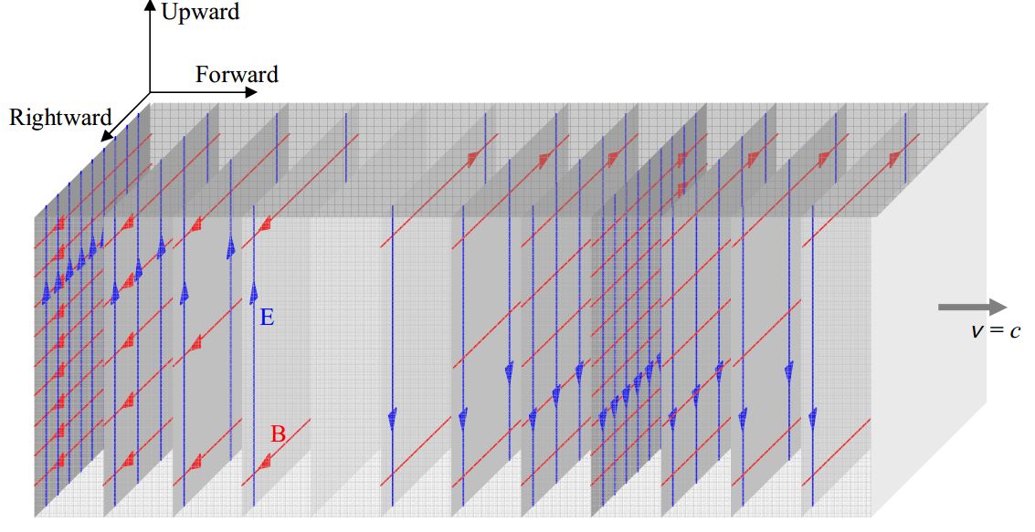
Each “sheet” in the diagram characterizes the electric (vertical arrows) and magnetic (horizontal arrows) fields at the instant in time depicted. On each sheet, we use the field diagram convention with which you are already familiar—the stronger the field, the more densely packed the field lines in the diagram.
Consider the one thin horizontal slice of the beam depicted in this diagram:
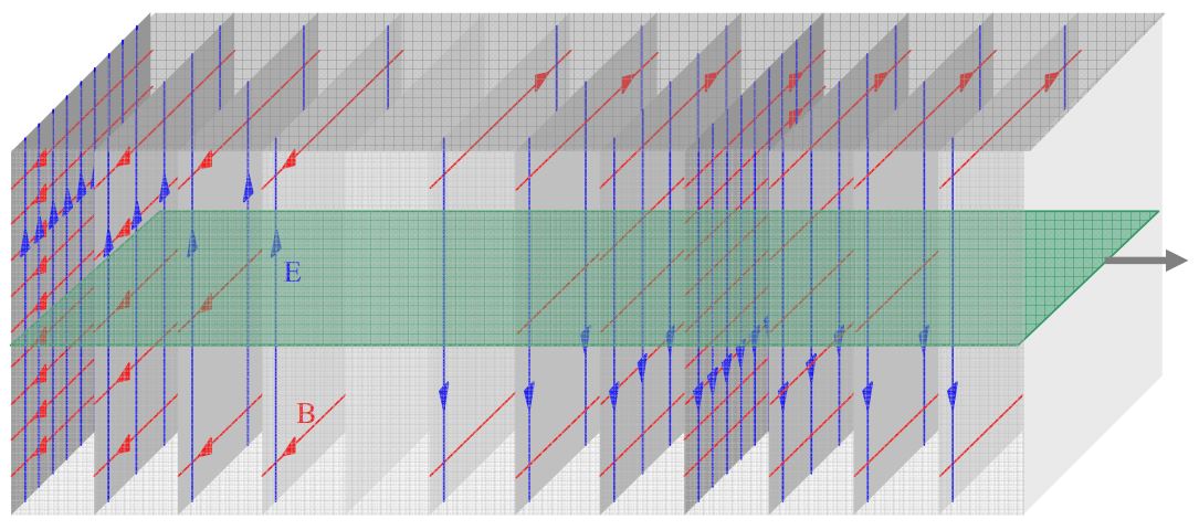
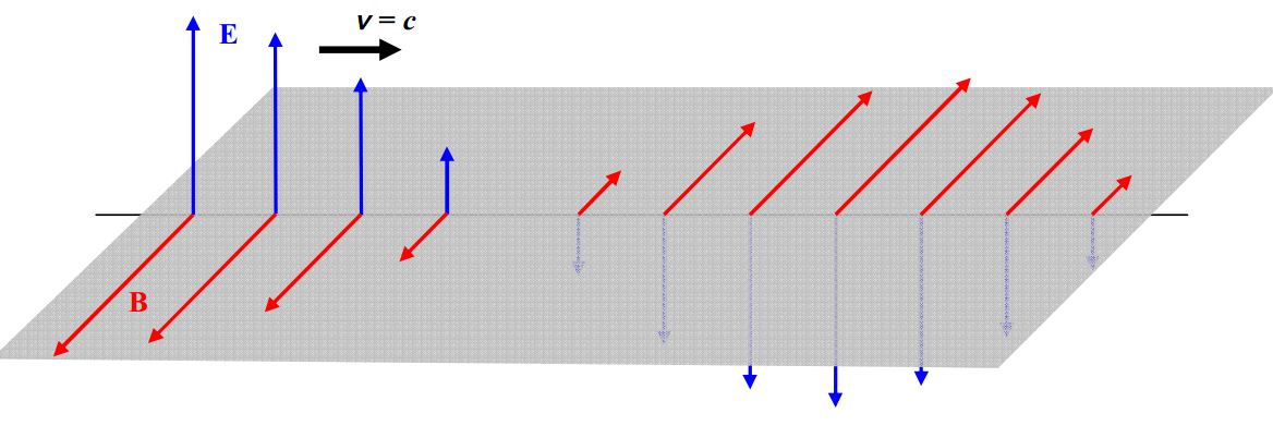
Here we depict the electric field on that one thin horizontal region:
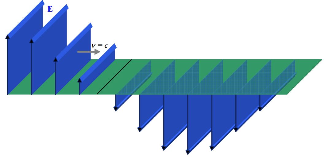
This is a simpler diagram with less information which is, perhaps, easier to interpret, but, also, perhaps, easier to misinterpret. It may for instance, be more readily apparent to you that what we are depicting (as we were in the other diagram) is just 34 of a wavelength of the wave. On the other hand, the diagram is more abstract—the length of the electric field vectors does not represent extent through space, but rather, the magnitude of the electric field at the tail of the arrow. As mentioned, the set of locations of the tails of the arrows, namely the horizontal plane, is the only place the diagram is giving information. It is generally assumed that the electric field has the same pattern for some distance above and below the plane on which it is specified in the diagram. Note the absence of the magnetic field. It is up to the reader to know that; as part of the light, there is a magnetic field wherever there is an electric field, and that, the greater the electric field, the greater the magnetic field, and that the magnetic field is perpendicular both to the direction in which the light is going, and to the electric field. (Recall that the direction of the magnetic field is such that the vector →E×→B is in the same direction as the velocity of the wave.)
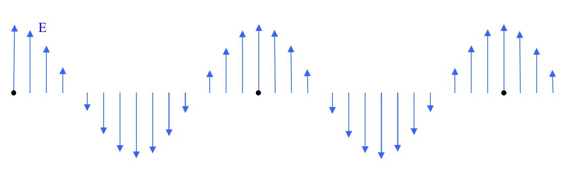
An example of an electric field depiction, on a single line along the direction of travel, would be:
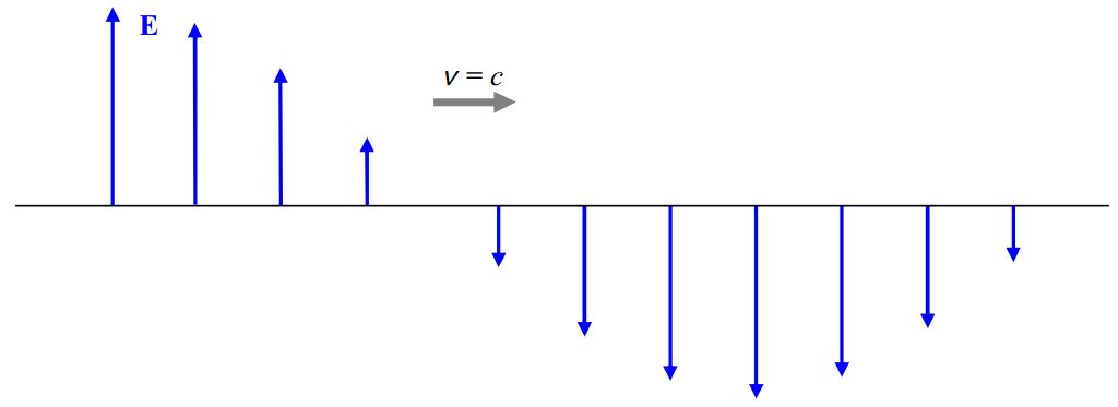
It is important to keep in mind that the arrows are characterizing the electric field at points on the one line, and, it’s the length of the arrow that indicates the strength of the electric field at the tail of the arrow, not the spacing between arrows.
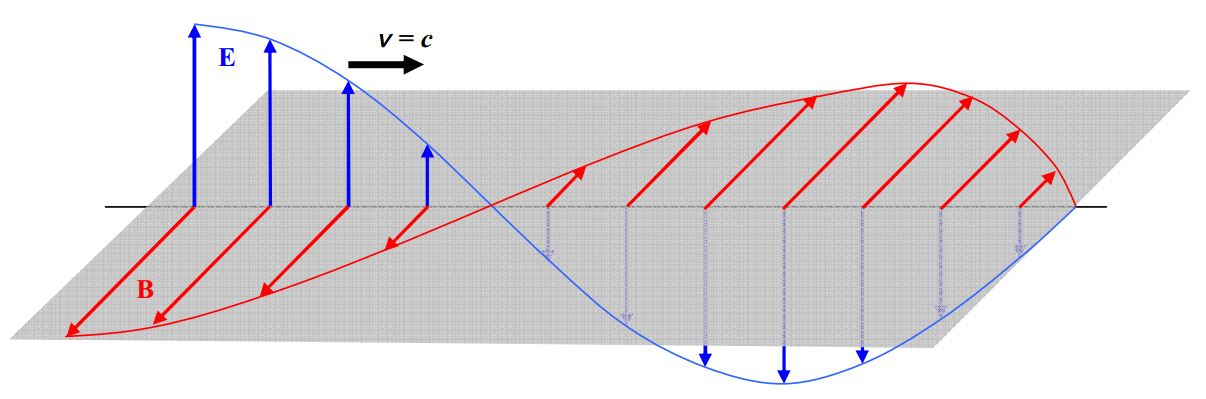
The simplicity of this field-on-a-line diagram allows for the inclusion of the magnetic field vectors in the same diagram:
If one connects the tips of the arrows in this kind of diagram, the meaning of those Electric Field vs. Position sinusoidal curves presented in the last chapter becomes more evident:
Huygens’ Principle involves wavefronts. A wavefront is the part of a wave which is at a surface that is everywhere perpendicular to the direction in which the wave is traveling. If such surfaces are planes, the wave is called a plane wave. The kind of wave we have been depicting is a plane wave. The set of fields on any one of the gray “sheets” on in the diagram:
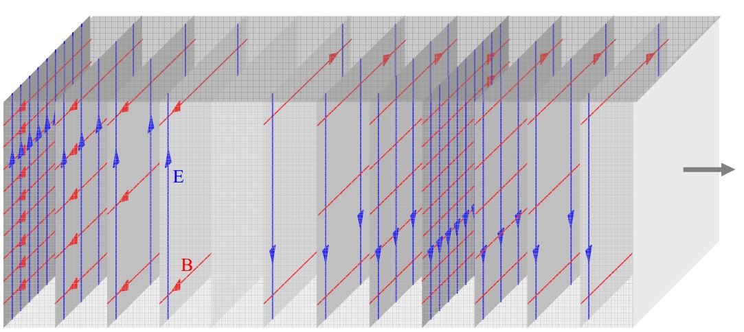
is a part of a wavefront. It is customary to focus our attention on wavefronts at which the electric and magnetic fields are a maximum in one direction. The rearmost sheet in the diagram above represents such a wavefront.
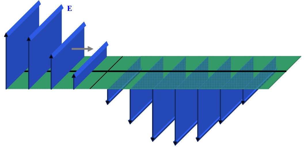
In the following diagram, you see black lines on the top of each sheet representing maximum-upward-directed-electric-field wavefronts.
And, in the following, each such wavefront is marked with a black dot:
A common method of depicting wavefronts corresponds to a view from above, of the preceding electric field sheet diagram which I copy here:

Such a wavefront diagram appears as:
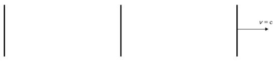
More commonly, you’ll see more of them packed closer together. The idea is that the wavefronts look like a bird’s eye view of waves in the ocean.
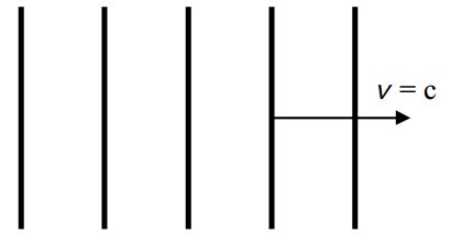
Note that the distance between adjacent maximum-field wavefronts, as depicted here, is one wavelength.
At this point we are ready to use the Huygens’s Principle idea, the notion of a wavefront, and our understanding of the way physicists depict wavefronts diagrammatically, to explore the phenomenon of two slit interference.