
3.3: Gravitational Phenomena


- Last updated
- Mar 12, 2024
- Save as PDF

( \newcommand{\kernel}{\mathrm{null}\,}\)
Cruise your radio dial today and try to find any popular song that would have been imaginable without Louis Armstrong. By introducing solo improvisation into jazz, Armstrong took apart the jigsaw puzzle of popular music and fit the pieces back together in a different way. In the same way, Newton reassembled our view of the universe. Consider the titles of some recent physics books written for the general reader: The God Particle, Dreams of a Final Theory. When the subatomic particle called the neutrino was recently proven for the first time to have mass, specialists in cosmology began discussing seriously what effect this would have on calculations of the evolution of the universe from the Big Bang to its present state. Without the English physicist Isaac Newton, such attempts at universal understanding would not merely have seemed ambitious, they simply would not have occurred to anyone.
This section is about Newton's theory of gravity, which he used to explain the motion of the planets as they orbited the sun. Newton tosses off a general treatment of motion in the first 20 pages of his Mathematical Principles of Natural Philosophy, and then spends the next 130 discussing the motion of the planets. Clearly he saw this as the crucial scientific focus of his work. Why? Because in it he showed that the same laws of nature applied to the heavens as to the earth, and that the gravitational interaction that made an apple fall was the same as the as the one that kept the earth's motion from carrying it away from the sun.
2.3.1 Kepler's laws
Newton wouldn't have been able to figure out why the planets move the way they do if it hadn't been for the astronomer Tycho Brahe (1546-1601) and his protege Johannes Kepler (1571-1630), who together came up with the first simple and accurate description of how the planets actually do move. The difficulty of their task is suggested by the figure below, which shows how the relatively simple orbital motions of the earth and Mars combine so that as seen from earth Mars appears to be staggering in loops like a drunken sailor.
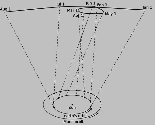
d / As the earth and Mars revolve around the sun at different rates, the combined effect of their motions makes Mars appear to trace a strange, looped path across the background of the distant stars.
Brahe, the last of the great naked-eye astronomers, collected extensive data on the motions of the planets over a period of many years, taking the giant step from the previous observations' accuracy of about 10 minutes of arc (10/60 of a degree) to an unprecedented 1 minute. The quality of his work is all the more remarkable considering that his observatory consisted of four giant brass protractors mounted upright in his castle in Denmark. Four different observers would simultaneously measure the position of a planet in order to check for mistakes and reduce random errors.
With Brahe's death, it fell to his former assistant Kepler to try to make some sense out of the volumes of data. After 900 pages of calculations and many false starts and dead-end ideas, Kepler finally synthesized the data into the following three laws:
Kepler's elliptical orbit law: The planets orbit the sun in elliptical orbits with the sun at one focus.
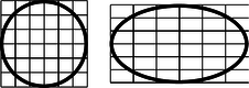
a / An ellipse is circle that has been distorted by shrinking and stretching along perpendicular axes.
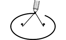
b / An ellipse can be constructed by tying a string to two pins and drawing like this with a pencil stretching the string taut. Each pin constitutes one focus of the ellipse.
Kepler's equal-area law: The line connecting a planet to the sun sweeps out equal areas in equal amounts of time.
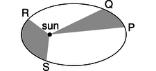
c / If the time interval taken by the planet to move from P to Q is equal to the time interval from R to S, then according to Kepler's equal-area law, the two shaded areas are equal. The planet is moving faster during time interval RS than it was during PQ, because gravitational energy has been transformed into kinetic energy.
Kepler's law of periods: The time required for a planet to orbit the sun, called its period, T, is proportional to the long axis of the ellipse raised to the 3/2 power. The constant of proportionality is the same for all the planets.
Although the planets' orbits are ellipses rather than circles, most are very close to being circular. The earth's orbit, for instance, is only flattened by 1.7% relative to a circle. In the special case of a planet in a circular orbit, the two foci (plural of “focus”) coincide at the center of the circle, and Kepler's elliptical orbit law thus says that the circle is centered on the sun. The equal-area law implies that a planet in a circular orbit moves around the sun with constant speed. For a circular orbit, the law of periods then amounts to a statement that the time for one orbit is proportional to r3/2, where r is the radius. If all the planets were moving in their orbits at the same speed, then the time for one orbit would simply depend on the circumference of the circle, so it would only be proportional to r to the first power. The more drastic dependence on r3/2 means that the outer planets must be moving more slowly than the inner planets.Our main focus in this section will be to use the law of periods to deduce the general equation for gravitational energy. The equal-area law turns out to be a statement on conservation of angular momentum, which is discussed in chapter 4. We'll demonstrate the elliptical orbit law numerically in chapter 3, and analytically in chapter 4.2.3.2 Circular orbits Kepler's laws say that planets move along elliptical paths (with circles as a special case), which would seem to contradict the proof on page 90 that objects moving under the influence of gravity have parabolic trajectories. Kepler was right. The parabolic path was really only an approximation, based on the assumption that the gravitational field is constant, and that vertical lines are all parallel. In figure e, trajectory 1 is an ellipse, but it gets chopped off when the cannonball hits the earth, and the small piece of it that is above ground is nearly indistinguishable from a parabola. Our goal is to connect the previous calculation of parabolic trajectories, y=(g/2v2)x2, with Kepler's data for planets orbiting the sun in nearly circular orbits. Let's start by thinking in terms of an orbit that circles the earth, like orbit 2 in figure e. It's more natural now to choose a coordinate system with its origin at the center of the earth, so the parabolic approximation becomes y=r−(g/2v2)x2, where r is the distance from the center of the earth. For small values of x, i.e., when the cannonball hasn't traveled very far from the muzzle of the gun, the parabola is still a good approximation to the actual circular orbit, defined by the Pythagorean theorem, r2=x2+y2, or y=r√1−x2/r2. For small values of x, we can use the approximation √1+ϵ≈1+ϵ/2 to find y≈r−(1/2r)x2. Setting this equal to the equation of the parabola, we have g/2v2=(1/2r), orv=√gr[condition for a circular orbit].
e / A cannon fires cannonballs at different velocities, from the top of an imaginary mountain that rises above the earth's atmosphere. This is almost the same as a figure Newton included in his Mathematical Principles.
| Example 14: Low-earth orbit |
|---|
| To get a feel for what this all means, let's calculate the velocity required for a satellite in a circular low-earth orbit. Real low-earth-orbit satellites are only a few hundred km up, so for purposes of rough estimation we can take r to be the radius of the earth, and g is not much less than its value on the earth's surface, 10 m/s2. Taking numerical data from Appendix 5, we havev=√gr=√(10 m/s2)(6.4×103 km)=√(10 m/s2)(6.4×106 m)=√6.4×10⁷ m2/s2=8000 m/s(about twenty times the speed of sound).In one second, the satellite moves 8000 m horizontally. During this time, it drops the same distance any other object would: about 5 m. But a drop of 5 m over a horizontal distance of 8000 m is just enough to keep it at the same altitude above the earth's curved surface. |
2.3.3 The sun's gravitational field
We can now use the circular orbit condition v=√gr, combined with Kepler's law of periods, T∝r3/2 for circular orbits, to determine how the sun's gravitational field falls off with distance.8 From there, it will be just a hop, skip, and a jump to get to a universal description of gravitational interactions.The velocity of a planet in a circular orbit is proportional to r/T, sor/T∝√grr/r3/2∝√grg∝1/r2If gravity behaves systematically, then we can expect the same to be true for the gravitational field created by any object, not just the sun.There is a subtle point here, which is that so far, r has just meant the radius of a circular orbit, but what we have come up with smells more like an equation that tells us the strength of the gravitational field made by some object (the sun) if we know how far we are from the object. In other words, we could reinterpret r as the distance from the sun.
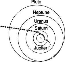
i / The Pioneer 10 space probe's trajectory from 1974 to 1992, with circles marking its position at one-year intervals. After its 1974 slingshot maneuver around Jupiter, the probe's motion was determined almost exclusively by the sun's gravity.
2.3.4 Gravitational energy in general
We now want to find an equation for the gravitational energy of any two masses that attract each other from a distance r. We assume that r is large enough compared to the distance between the objects so that we don't really have to worry about whether r is measured from center to center or in some other way. This would be a good approximation for describing the solar system, for example, since the sun and planets are small compared to the distances between them --- that's why you see Venus (the “evening star”) with your bare eyes as a dot, not a disk.
The equation we seek is going to give the gravitational energy, U, as a function of m1, m2, and r. We already know from experience with gravity near the earth's surface that U is proportional to the mass of the object that interacts with the earth gravitationally, so it makes sense to assume the relationship is symmetric: U is presumably proportional to the product m1m2. We can no longer assume ΔU∝Δr, as in the earth's-surface equation ΔU=mgΔy, since we are trying to construct an equation that would be valid for all values of r, and g depends on r. We can, however, consider an infinitesimally small change in distance dr, for which we'll have dU=m2g1dr, where g1 is the gravitational field created by m1. (We could just as well have written this as dU=m1g2dr, since we're not assuming either mass is “special” or “active.”) Integrating this equation, we have
where we're free to take the constant of integration to be equal to zero, since gravitational energy is never a well-defined quantity in absolute terms. Writing G for the constant of proportionality, we have the following fundamental description of gravitational interactions:
We'll refer to this as Newton's law of gravity, although in reality he stated it in an entirely different form, which turns out to be mathematically equivalent to this one.
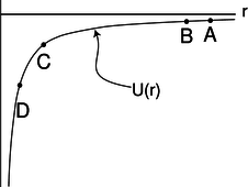
f / The gravitational energy U=−Gm1m2/r graphed as a function of r.
Let's interpret his result. First, don't get hung up on the fact that it's negative, since it's only differences in gravitational energy that have physical significance. The graph in figure f could be shifted up or down without having any physical effect. The slope of this graph relates to the strength of the gravitational field. For instance, suppose figure f is a graph of the gravitational energy of an asteroid interacting with the sun. If the asteroid drops straight toward the sun, from A to B, the decrease in gravitational energy is very small, so it won't speed up very much during that motion. Points C and D, however, are in a region where the graph's slope is much greater. As the asteroid moves from C to D, it loses a lot of gravitational energy, and therefore speeds up considerably. This is due to the stronger gravitational field.
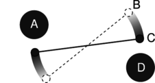
| Example 15: Determining G |
|---|
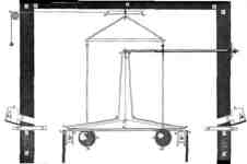
| The constant G is not easy to determine, and Newton went to his grave without knowing an accurate value for it. If we knew the mass of the earth, then we could easily determine G from experiments with terrestrial gravity, but the only way to determine the mass of the earth accurately in units of kilograms is by finding G and reasoning the other way around! (If you estimate the average density of the earth, you can make at least a rough estimate of G.) Figures g and h show how G was first measured by Henry Cavendish in the nineteenth century.The rotating arm is released from rest, and the kinetic energy of the two moving balls is measured when they pass position C. Conservation of energy gives −2GMmrBA−2GMmrBD=−2GMmrCA−2GMmrCD+2K, where M is the mass of one of the large balls, m is the mass of one of the small ones, and the factors of two, which will cancel, occur because every energy is mirrored on the opposite side of the apparatus. (As discussed on page 102, it turns out that we get the right result by measuring all the distances from the center of one sphere to the center of the other.) This can easily be solved for G. The best modern value of G, from later versions of the same experiment, is 6.67×10⁻¹¹ J⋅m/kg2.
g / Cavendish's original drawing of the apparatus for his experiment, discussed in example 15. The room was sealed to exclude air currents, and the motion was observed through telescopes sticking through holes in the walls.
h / A simplified drawing of the Cavendish experiment, viewed from above. The rod with the two small masses on the ends hangs from a thin fiber, and is free to rotate.
|
| Example 16: Escape velocity |
|---|
| ▹ The Pioneer 10 space probe was launched in 1972, and continued sending back signals for 30 years. In the year 2001, not long before contact with the probe was lost, it was about 1.2×10¹³ m from the sun, and was moving almost directly away from the sun at a velocity of 1.21×10⁴ m. The mass of the sun is 1.99×1030 kg. Will Pioneer 10 escape permanently, or will it fall back into the solar system? ▹ We want to know whether there will be a point where the probe will turn around. If so, then it will have zero kinetic energy at the turnaround point: Ki+Ui=Uf12mv2−GMmri=−GMmrf12v2−GMri=−GMrf, where M is the mass of the sun, m is the (irrelevant) mass of the probe, and rf is the distance from the sun of the hypothetical turnaround point. Plugging in numbers on the left, we get a positive result. There can therefore be no solution, since the right side is negative. There won't be any turnaround point, and Pioneer 10 is never coming back. The minimum velocity required for this to happen is called escape velocity. For speeds above escape velocity, the orbits are open-ended hyperbolas, rather than repeating elliptical orbits. In figure i, Pioneer's hyperbolic trajectory becomes almost indistinguishable from a line at large distances from the sun. The motion slows perceptibly in the first few years after 1974, but later the speed becomes nearly constant, as shown by the nearly constant spacing of the dots. |
The gravitational field
We got the energy equation U=−Gm1m2/r by integrating g∝1/r2 and then inserting a constant of proportionality to make the proportionality into an equation. The opposite of an integral is a derivative, so we can now go backwards and insert a constant of proportionality in g∝1/r2 that will be consistent with the energy equation:
This kind of inverse-square law occurs all the time in nature. For instance, if you go twice as far away from a lightbulb, you receive 1/4 as much light from it, because as the light spreads out, it is like an expanding sphere, and a sphere with twice the radius has four times the surface area. It's like spreading the same amount of peanut butter on four pieces of bread instead of one --- we have to spread it thinner.
Discussion Questions
◊ A bowling ball interacts gravitationally with the earth. Would it make sense for the gravitational energy to be inversely proportional to the distance between their surfaces rather than their centers?
2.3.5 The shell theorem
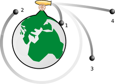
Newton's great insight was that gravity near the earth's surface was the same kind of interaction as the one that kept the planets from flying away from the sun. He told his niece that the idea came to him when he saw an apple fall from a tree, which made him wonder whether the earth might be affecting the apple and the moon in the same way. Up until now, we've generally been dealing with gravitational interactions between objects that are small compared to the distances between them, but that assumption doesn't apply to the apple. A kilogram of dirt a few feet under his garden in England would interact much more strongly with the apple than a kilogram of molten rock deep under Australia, thousands of miles away. Also, we know that the earth has some parts that are more dense, and some parts that are less dense. The solid crust, on which we live, is considerably less dense than the molten rock on which it floats. By all rights, the computation of the total gravitational energy of the apple should be a horrendous mess. Surprisingly, it turns out to be fairly simple in the end. First, we note that although the earth doesn't have the same density throughout, it does have spherical symmetry: if we imagine dividing it up into thin concentric shells, the density of each shell is uniform.
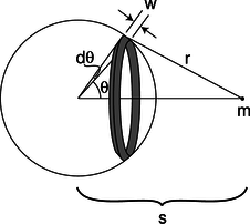
j / A spherical shell of mass M interacts with a pointlike mass m.
Second, it turns out that a uniform spherical shell interacts with external masses as if all its mass were concentrated at its center.
\mythmhdr{The shell theorem} The gravitational energy of a uniform spherical shell of mass M interacting with a pointlike mass m outside it equals −GMm/s, where s is the center-to-center distance. If mass m is inside the shell, then the energy is constant, i.e., the shell's interior gravitational field is zero.
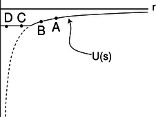
k / The gravitational energy of a mass m at a distance s from the center of a hollow spherical shell of mass.
\mythmhdr{Proof} Let b be the radius of the shell, h its thickness, and ρ its density. Its volume is then V=(area)(thickness)=4πb2h, and its mass is M=ρV=4πρb2h. The strategy is to divide the shell up into rings as shown in figure j, with each ring extending from θ to θ+dθ. Since the ring is infinitesimally skinny, its entire mass lies at the same distance, r, from mass m. The width of such a ring is found by the definition of radian measure to be w=bdθ, and its mass is dM=(ρ)(circumference)(thickness)(width)= (ρ)(2πbsinθ)(h)(bdθ)=2πρb2hsinθdθ. The gravitational energy of the ring interacting with mass m is therefore
The integral has a mixture of the variables r and θ, which are related by the law of cosines,
and to evaluate the integral, we need to get everything in terms of either r and dr or θ and dθ. The relationship between the differentials is found by differentiating the law of cosines,
and since sinθdθ occurs in the integral, the easiest path is to substitute for it, and get everything in terms of r and dr:
This was all under the assumption that mass m was on the outside of the shell. To complete the proof, we consider the case where it's inside. In this case, the only change is that the limits of integration are different:
The two results are equal at the surface of the sphere, s=b, so the constant-energy part joins continuously onto the 1/s part, and the effect is to chop off the steepest part of the graph that we would have had if the whole mass M had been concentrated at its center. Dropping a mass m from A to B in figure k releases the same amount of energy as if mass M had been concentrated at its center, but there is no release of gravitational energy at all when moving between two interior points like C and D. In other words, the internal gravitational field is zero. Moving from C to D brings mass m farther away from the nearby side of the shell, but closer to the far side, and the cancellation between these two effects turns out to be perfect. Although the gravitational field has to be zero at the center due to symmetry, it's much more surprising that it cancels out perfectly in the whole interior region; this is a special mathematical characteristic of a 1/r interaction like gravity.
| Example 17: Newton's apple |
|---|
| Over a period of 27.3 days, the moon travels the circumference of its orbit, so using data from Appendix 5, we can calculate its speed, and solve the circular orbit condition to determine the strength of the earth's gravitational field at the moon's distance from the earth, g=v2/r=2.72×10−3 m/s2, which is 3600 times smaller than the gravitational field at the earth's surface. The center-to-center distance from the moon to the earth is 60 times greater than the radius of the earth. The earth is, to a very good approximation, a sphere made up of concentric shells, each with uniform density, so the shell theorem tells us that its external gravitational field is the same as if all its mass was concentrated at its center. We already know that a gravitational energy that varies as −1/r is equivalent to a gravitational field proportional to 1/r2, so it makes sense that a distance that is greater by a factor of 60 corresponds to a gravitational field that is 60×60=3600 times weaker. Note that the calculation didn't require knowledge of the earth's mass or the gravitational constant, which Newton didn't know. In 1665, shortly after Newton graduated from Cambridge, the Great Plague forced the college to close for two years, and Newton returned to the family farm and worked intensely on scientific problems. During this productive period, he carried out this calculation, but it came out wrong, causing him to doubt his new theory of gravity. The problem was that during the plague years, he was unable to use the university's library, so he had to use a figure for the radius of the moon's orbit that he had memorized, and he forgot that the memorized value was in units of nautical miles rather than statute miles. Once he realized his mistake, he found that the calculation came out just right, and became confident that his theory was right after all. 9 |
| Example 18: Weighing the earth |
|---|
| ▹ Once Cavendish had found G=6.67×10⁻¹¹ J⋅m/kg2 (p. 101, example 15), it became possible to determine the mass of the earth. By the shell theorem, the gravitational energy of a mass m at a distance r from the center of the earth is U=−GMm/r, where M is the mass of the earth. The gravitational field is related to this by mgdr=dU, or g=(1/m)dU/dr=GM/r2. Solving for M, we have M=gr2/G=(9.8\ m/s2)(6.4×106\ m)26.67×10⁻¹¹ J⋅m/kg2=6.0×1024 m2⋅kg2J⋅s2=6.0×1024 kg |
| Example 19: Gravity inside the earth |
|---|
| ▹ The earth is somewhat more dense at greater depths, but as an approximation let's assume it has a constant density throughout. How does its internal gravitational field vary with the distance r from the center? ▹ Let's write b for the radius of the earth. The shell theorem tell us that at a given location r, we only need to consider the mass M<r that is deeper than r. Under the assumption of constant density, this mass is related to the total mass of the earth by M<rM=r3b3, and by the same reasoning as in example 18, g=GM<rr2, so g=GMrb3. In other words, the gravitational field interpolates linearly between zero at r=0 and its ordinary surface value at r=b. |
The following example applies the numerical techniques of section 2.2.
| Example 20: From the earth to the moon | ||||
|---|---|---|---|---|
|
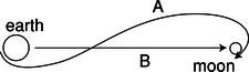
l / The actual trajectory of the Apollo 11 spacecraft, A, and the straight-line trajectory, B, assumed in the example.
The Apollo 11 mission landed the first humans on the moon in 1969. In this example, we'll estimate the time it took to get to the moon, and compare our estimate with the actual time, which was 73.0708 hours from the engine burn that took the ship out of earth orbit to the engine burn that inserted it into lunar orbit. During this time, the ship was coasting with the engines off, except for a small course-correction burn, which we neglect. More importantly, we do the calculation for a straight-line trajectory rather than the real S-shaped one, so the result can only be expected to agree roughly with what really happened. The following data come from the original press kit, which NASA has scanned and posted on the Web:
The endpoint of the the straight-line trajectory is a free-fall impact on the lunar surface, which is also unrealistic (luckily for the astronauts). The ship's energy is E=−GMemr−GMmmrm−r+12mv2,but since everything is proportional to the mass of the ship, m, we can divide it outEm=−GMer−GMmrm−r+12v2,
and the energy variables in the program with names like e, k, and u are actually energies per unit mass. The program is a straightforward modification of the function time3 on page 93. import math
def tmoon(vi,ri,rf,n):
bigg=6.67e-11 # gravitational constant
me=5.97e24 # mass of earth
mm=7.35e22 # mass of moon
rm=3.84e8 # earth-moon distance
r=ri
v=vi
dr = (rf-ri)/n
e=-bigg*me/ri-bigg*mm/(rm-ri)+.5*vi**2
t=0
for i in range(n):
u_old = -bigg*me/r-bigg*mm/(rm-r)
k_old = e - u_old
v_old = math.sqrt(2.*k_old)
r = r+dr
u = -bigg*me/r-bigg*mm/(rm-r)
k = e - u
v = math.sqrt(2.*k)
v_avg = .5*(v_old+v)
dt=dr/v_avg
t=t+dt
return t
>>> re=6.378e6  # radius of earth
>>> rm=1.74e6   # radius of moon
>>> ri=re+3.363e5       # re+initial altitude
>>> rf=3.8e8-rm # earth-moon distance minus rm
>>> vi=1.083e4 # initial velocity
>>> print(tmoon(vi,ri,rf,1000)/3600.) # convert seconds to hours
59.654047441976552
This is pretty decent agreement, considering the wildly inaccurate trajectory assumed. It's interesting to see how much the duration of the trip changes if we increase the initial velocity by only ten percent: >>> vi=1.2e4 >>> print(tmoon(vi,ri,rf,1000)/3600.) 18.177752636111677 The most important reason for using the lower speed was that if something had gone wrong, the ship would have been able to whip around the moon and take a “free return” trajectory back to the earth, without having to do any further burns. At a higher speed, the ship would have had so much kinetic energy that in the absence of any further engine burns, it would have escaped from the earth-moon system. The Apollo 13 mission had to take a free return trajectory after an explosion crippled the spacecraft. |
Contributors and Attributions
Benjamin Crowell (Fullerton College). Conceptual Physics is copyrighted with a CC-BY-SA license.