8.1: Introduction

Last updated
Save as PDF

Page ID: 6974

\( \newcommand{\vecs}[1]{\overset { \scriptstyle \rightharpoonup} {\mathbf{#1}} } \) \( \newcommand{\vecd}[1]{\overset{-\!-\!\rightharpoonup}{\vphantom{a}\smash {#1}}} \)\(\newcommand{\id}{\mathrm{id}}\) \( \newcommand{\Span}{\mathrm{span}}\) \( \newcommand{\kernel}{\mathrm{null}\,}\) \( \newcommand{\range}{\mathrm{range}\,}\) \( \newcommand{\RealPart}{\mathrm{Re}}\) \( \newcommand{\ImaginaryPart}{\mathrm{Im}}\) \( \newcommand{\Argument}{\mathrm{Arg}}\) \( \newcommand{\norm}[1]{\| #1 \|}\) \( \newcommand{\inner}[2]{\langle #1, #2 \rangle}\) \( \newcommand{\Span}{\mathrm{span}}\) \(\newcommand{\id}{\mathrm{id}}\) \( \newcommand{\Span}{\mathrm{span}}\) \( \newcommand{\kernel}{\mathrm{null}\,}\) \( \newcommand{\range}{\mathrm{range}\,}\) \( \newcommand{\RealPart}{\mathrm{Re}}\) \( \newcommand{\ImaginaryPart}{\mathrm{Im}}\) \( \newcommand{\Argument}{\mathrm{Arg}}\) \( \newcommand{\norm}[1]{\| #1 \|}\) \( \newcommand{\inner}[2]{\langle #1, #2 \rangle}\) \( \newcommand{\Span}{\mathrm{span}}\)\(\newcommand{\AA}{\unicode[.8,0]{x212B}}\)

As it goes about its business, a particle may experience many different sorts of forces. In Chapter 7, we looked at the effect of forces that depend only on the speed of the particle. In a later chapter we shall look at forces that depend only on the position of the particle. (Such forces will be called conservative forces.) In this chapter we shall look at the effect of forces that vary with time. Of course, it is quite possible that an unfortunate particle may be buffeted by forces that depend on its speed, on its position, and on the time - but, as far as this chapter is concerned, we shall be looking at forces that depend only on the time.

Everyone knows that Newton's second law of motion states that when a force acts on a body, the momentum of the body changes, and the rate of change of momentum is equal to the applied force. That is, \( F=\frac{dp}{dt}\). If a force that varies with time, \( F(t)\), acts on a body for a time \( T\), the integral of the force over the time, \( \int_{0}^{T}F(t)dt \) is called the impulse of the force, and it results in a change of momentum \( \Delta P \) which is equal to the impulse. I shall use the symbol \( J\) to represent impulse, or the time integral of a force. Its SI units would be N s, and its dimensions MLT^-1, which is the same as the dimensions of momentum.

Thus, Newton's second law of motion is

\[ F=\dot{p}. \nonumber \]

When integrated over time, this becomes

\[ J=\Delta p. \nonumber \]

Likewise, in rotational motion, the angular momentum \( L\) of a body changes when a torque \( \tau\) acts on it, such that the rate of change of angular momentum is equal to the applied torque:

\[ \tau = \dot{L}. \nonumber \]

If the torque, which may vary with time, acts over a time \( T\), the integral of the torque over the time, \( \int_{0}^{T}\tau dt \) is the angular impulse, which I shall denote by the symbol \( K\), and it results in a change of the angular momentum:

\[ K =\Delta L. \nonumber \]

The SI units of angular impulse are N m s, and the dimensions are ML²T^-1, which are the same as those of angular momentum.

For example, suppose that a golf ball is struck by a force varies with time as

\[ F = \hat{F}\left[1-\left(\frac{|t-t_{0}|}{\tau}\right)^{\frac{2}{3}}\right]^{\frac{3}{2}} \nonumber \]

This may look like a highly-contrived and unlikely function, but in Figure VIII.1 I have drawn it for \( \hat{F}=1\), \( t_{0}=3\), \( \tau=1\) and you will see that it is a reasonably plausible function. The club is in contact with the ball from time \( t_{0}-\tau\) to \( t_{0}+\tau\).

alt

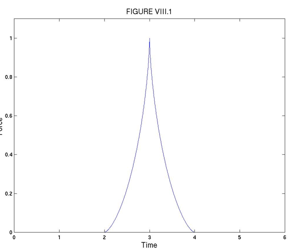
If the ball, of mass \( m\), starts from rest, what will be its speed \( V\) immediately after it leaves the club? The answer is that its new momentum, \( mV\), will equal the impulse (or the time integral) of the above force:

\[ mV = \hat{F}\int_{t_{0}-\tau}^{t_{0}+\tau}\left[1-\left(\frac{|t-t_{0}|}{\tau}\right)^{\frac{2}{3}}\right]^{\frac{3}{2}}dt. \nonumber \]

This is very easy to understand; if there is any difficulty it might be in the mechanics of working out this integral. It is good integration practice, but, if you can't do it after a reasonable effort, and you want a hint, ask me (jtatum@uvic.ca) and I'll see what I can do. You should get

\[ mV = \frac{3\pi}{16}\hat{F}\tau =0.589\hat{F}\tau \nonumber \]

Example \(\PageIndex{1}\)

Here is a very similar example, except that the integration is rather easier. A ball of mass 500 g, initially at rest, is struck with a force that varies with time as

\(F = \hat{F}\left[1-\left(\frac{t-t_{0}}{\tau}\right)^{2}\right]^{\frac{1}{2}}\),

where \( \hat{F}\) = 4000N, \( t_{0}\) = 10 ms, \( t\) = 3 ms. Draw (accurately, by computer) a graph of \( F\) versus time (it doesn't look quite like Figure VIII.1). How fast is the ball moving immediately after impact?

(I make it 37.7 m s^-1.)