
5.7: Pauli Two-Component Formalism

( \newcommand{\kernel}{\mathrm{null}\,}\)
We have seen, in Section 4.4, that the eigenstates of orbital angular momentum can be conveniently represented as spherical harmonics. In this representation, the orbital angular momentum operators take the form of differential operators involving only angular coordinates. It is conventional to represent the eigenstates of spin angular momentum as column (or row) matrices. In this representation, the spin angular momentum operators take the form of matrices.
The matrix representation of a spin one-half system was introduced by Pauli in 1926. Recall, from Section 5.4, that a general spin ket can be expressed as a linear combination of the two eigenkets of Sz belonging to the eigenvalues |±⟩ . Let us represent these basis eigenkets as column vectors:
→(10)≡χ+, ??? →(01)≡χ−. ???The corresponding eigenbras are represented as row vectors:
→(1,0)≡χ\dag+, ??? →(0,1)≡χ\dag−. ???In this scheme, a general ket takes the form
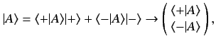 ???
??? and a general bra becomes
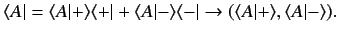 ???
??? The column vector ??? is called a two-component spinor, and can be written
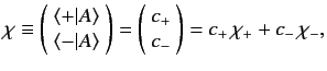 ???
??? where the c± are complex numbers. The row vector ??? becomes
Consider the ket obtained by the action of a spin operator on ket A :
|A′⟩→(⟨+|A′⟩⟨−|A′⟩)≡χ′. ???However,
=⟨+|Sk|+⟩⟨+|A⟩+⟨+|Sk|−⟩⟨−|A⟩, ??? =⟨−|Sk|+⟩⟨+|A⟩+⟨−|Sk|−⟩⟨−|A⟩, ???or
![$ \left(\!\begin{array}{c}\langle +\vert A'\rangle\\ [0.5ex] \langl...
...}\langle +\vert A\rangle\\ [0.5ex] \langle -\vert A\rangle\end{array}\!\right).$](http://farside.ph.utexas.edu/teaching/qm/lectures/img1161.png) ???
??? It follows that we can represent the operator/ket relation ??? as the matrix relation
σk are the matrices of the ℏ/2 . These matrices, which are called the Pauli matrices, can easily be evaluated using the explicit forms for the spin operators given in Equations ???-???. We find that =(0110), ??? =(0−ii0), ??? =(100−1). ???Here, 1, 2, and 3 refer to y , and Sk→(ℏ2)σk.
???The expectation value of Sk can be written in terms of spinors and the Pauli matrices:
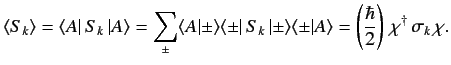 ???
??? The fundamental commutation relation for angular momentum, Equation ???, can be combined with ??? to give the following commutation relation for the Pauli matrices:
× =2i. ???It is easily seen that the matrices ???-??? actually satisfy these relations (i.e., {σi,σj}=2δij. ???
Here, |x′,y′,z′,±⟩=|x′,y′,z′⟩|±⟩=|±⟩|x′,y′,z′⟩. ???
The ket corresponding to state A is denoted A is completely specified by the two wavefunctions
=⟨x′,y′,z′|⟨+||A⟩⟩, ??? =⟨x′,y′,z′|⟨−||A⟩⟩. ???Consider the operator relation
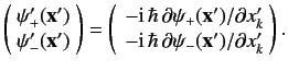
⟨x′,y′,z′|⟨+|A′⟩⟩where use has been made of the fact that the spin operator ⟨x′,y′,z′| . It is fairly obvious that we can represent the operator relation ??? as a matrix relation if we generalize our definition of a spinor by writing
χ′=(ℏ2)σkχ. ???Consider the operator relation
⟨x′,y′,z′|⟨+|A′⟩⟩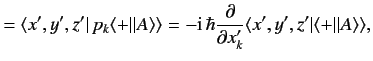 ??? ⟨x′,y′,z′|⟨−|A′⟩⟩
 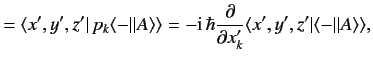 ???
??? where use has been made of Equation ???. The above equation reduces to
 ???
??? Thus, the operator equation ??? can be written
pk→−iℏ∂∂x′k1. ???Here, 1 is the pk or 2×2 unit matrix.
What about combinations of position and spin operators? The most commonly occurring combination is a dot product: e.g., σ ⋅L
. Consider the hybrid operator ⋅a , where 2×2 matrix: \boldmathσ![$ \cdot {\bf a} \equiv \sum_k a_k \,\sigma_k = \left(\!\begin{array...
...3 & a_1 -{\rm i}\,a_2\\ [0.5ex] a_1 + {\rm i}\,a_2 & -a_3 \end{array}\!\right).$](http://farside.ph.utexas.edu/teaching/qm/lectures/img1203.png) ???
??? Since, in the Schrödinger representation, a general position operator takes the form of a differential operator in y′ , or (⋅a)(⋅b)=a⋅b+i⋅(a×b) ???
follows from the commutation and anti-commutation relations ??? and ???. Thus,
=∑j∑k(12{σj,σk}+12[σj,σk])ajbk =a⋅b+i⋅(a×b). ???A general rotation operator in spin space is written
n is a unit vector pointing along the axis of rotation, and n can be regarded as a trivial position operator. The rotation operator is represented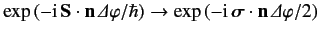 ???
??? in the Pauli scheme. The term on the right-hand side of the above expression is the exponential of a matrix. This can easily be evaluated using the Taylor series for an exponential, plus the rules
\( \mbox{\boldmath\)=1 , ??? \( \mbox{\boldmath\)=(⋅n) . ???These rules follow trivially from the identity ???. Thus, we can write
exp(−i\boldmathσ⋅nΔφ/2)![$ = \left[ 1 - \frac{(\mbox{\boldmath$\sigma$}\cdot {\bf n})^2}{2!}...
...t {\bf n})^4}{4!} \left(\frac{{\mit\Delta}\varphi}{2} \right)^4 + \cdots\right]$](http://farside.ph.utexas.edu/teaching/qm/lectures/img1224.png)
![$ - {\rm i} \left[ (\mbox{\boldmath$\sigma$}\cdot {\bf n} )\left( \...
...ot {\bf n})^3}{3!} \left(\frac{{\mit\Delta}\varphi}{2}\right)^3 + \cdots\right]$](http://farside.ph.utexas.edu/teaching/qm/lectures/img1225.png) \( \mbox{\boldmath\)2×2 form of this matrix is
\( \mbox{\boldmath\)2×2 form of this matrix is 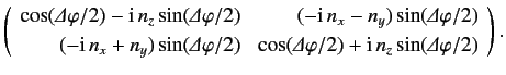 ???
??? Rotation matrices act on spinors in much the same manner as the corresponding rotation operators act on state kets. Thus,
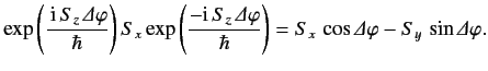
χ′ denotes the spinor obtained after rotating the spinor Δφ about the n -axis. The Pauli matrices remain unchanged under rotations. However, the quantity Sk [see Equation ???], so we would expect it to transform like a vector under rotation (see Section 5.4). In fact, we require Rkl are the elements of a conventional rotation matrix. This is easily demonstrated, because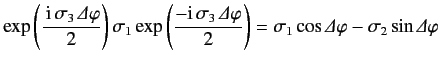 ???
??? plus all cyclic permutations. The above expression is the 2×2 matrix analogue of (see Section 5.4)
 ???
??? The previous two formulae can both be validated using the Baker-Hausdorff lemma, ???, which holds for Hermitian matrices, in addition to Hermitian operators.
Contributors
Richard Fitzpatrick (Professor of Physics, The University of Texas at Austin)