
9.2: Fundamental
- Page ID
- 1239

\( \newcommand{\vecs}[1]{\overset { \scriptstyle \rightharpoonup} {\mathbf{#1}} } \)
\( \newcommand{\vecd}[1]{\overset{-\!-\!\rightharpoonup}{\vphantom{a}\smash {#1}}} \)
\( \newcommand{\dsum}{\displaystyle\sum\limits} \)
\( \newcommand{\dint}{\displaystyle\int\limits} \)
\( \newcommand{\dlim}{\displaystyle\lim\limits} \)
\( \newcommand{\id}{\mathrm{id}}\) \( \newcommand{\Span}{\mathrm{span}}\)
( \newcommand{\kernel}{\mathrm{null}\,}\) \( \newcommand{\range}{\mathrm{range}\,}\)
\( \newcommand{\RealPart}{\mathrm{Re}}\) \( \newcommand{\ImaginaryPart}{\mathrm{Im}}\)
\( \newcommand{\Argument}{\mathrm{Arg}}\) \( \newcommand{\norm}[1]{\| #1 \|}\)
\( \newcommand{\inner}[2]{\langle #1, #2 \rangle}\)
\( \newcommand{\Span}{\mathrm{span}}\)
\( \newcommand{\id}{\mathrm{id}}\)
\( \newcommand{\Span}{\mathrm{span}}\)
\( \newcommand{\kernel}{\mathrm{null}\,}\)
\( \newcommand{\range}{\mathrm{range}\,}\)
\( \newcommand{\RealPart}{\mathrm{Re}}\)
\( \newcommand{\ImaginaryPart}{\mathrm{Im}}\)
\( \newcommand{\Argument}{\mathrm{Arg}}\)
\( \newcommand{\norm}[1]{\| #1 \|}\)
\( \newcommand{\inner}[2]{\langle #1, #2 \rangle}\)
\( \newcommand{\Span}{\mathrm{span}}\) \( \newcommand{\AA}{\unicode[.8,0]{x212B}}\)
\( \newcommand{\vectorA}[1]{\vec{#1}} % arrow\)
\( \newcommand{\vectorAt}[1]{\vec{\text{#1}}} % arrow\)
\( \newcommand{\vectorB}[1]{\overset { \scriptstyle \rightharpoonup} {\mathbf{#1}} } \)
\( \newcommand{\vectorC}[1]{\textbf{#1}} \)
\( \newcommand{\vectorD}[1]{\overrightarrow{#1}} \)
\( \newcommand{\vectorDt}[1]{\overrightarrow{\text{#1}}} \)
\( \newcommand{\vectE}[1]{\overset{-\!-\!\rightharpoonup}{\vphantom{a}\smash{\mathbf {#1}}}} \)
\( \newcommand{\vecs}[1]{\overset { \scriptstyle \rightharpoonup} {\mathbf{#1}} } \)
\(\newcommand{\longvect}{\overrightarrow}\)
\( \newcommand{\vecd}[1]{\overset{-\!-\!\rightharpoonup}{\vphantom{a}\smash {#1}}} \)
\(\newcommand{\avec}{\mathbf a}\) \(\newcommand{\bvec}{\mathbf b}\) \(\newcommand{\cvec}{\mathbf c}\) \(\newcommand{\dvec}{\mathbf d}\) \(\newcommand{\dtil}{\widetilde{\mathbf d}}\) \(\newcommand{\evec}{\mathbf e}\) \(\newcommand{\fvec}{\mathbf f}\) \(\newcommand{\nvec}{\mathbf n}\) \(\newcommand{\pvec}{\mathbf p}\) \(\newcommand{\qvec}{\mathbf q}\) \(\newcommand{\svec}{\mathbf s}\) \(\newcommand{\tvec}{\mathbf t}\) \(\newcommand{\uvec}{\mathbf u}\) \(\newcommand{\vvec}{\mathbf v}\) \(\newcommand{\wvec}{\mathbf w}\) \(\newcommand{\xvec}{\mathbf x}\) \(\newcommand{\yvec}{\mathbf y}\) \(\newcommand{\zvec}{\mathbf z}\) \(\newcommand{\rvec}{\mathbf r}\) \(\newcommand{\mvec}{\mathbf m}\) \(\newcommand{\zerovec}{\mathbf 0}\) \(\newcommand{\onevec}{\mathbf 1}\) \(\newcommand{\real}{\mathbb R}\) \(\newcommand{\twovec}[2]{\left[\begin{array}{r}#1 \\ #2 \end{array}\right]}\) \(\newcommand{\ctwovec}[2]{\left[\begin{array}{c}#1 \\ #2 \end{array}\right]}\) \(\newcommand{\threevec}[3]{\left[\begin{array}{r}#1 \\ #2 \\ #3 \end{array}\right]}\) \(\newcommand{\cthreevec}[3]{\left[\begin{array}{c}#1 \\ #2 \\ #3 \end{array}\right]}\) \(\newcommand{\fourvec}[4]{\left[\begin{array}{r}#1 \\ #2 \\ #3 \\ #4 \end{array}\right]}\) \(\newcommand{\cfourvec}[4]{\left[\begin{array}{c}#1 \\ #2 \\ #3 \\ #4 \end{array}\right]}\) \(\newcommand{\fivevec}[5]{\left[\begin{array}{r}#1 \\ #2 \\ #3 \\ #4 \\ #5 \\ \end{array}\right]}\) \(\newcommand{\cfivevec}[5]{\left[\begin{array}{c}#1 \\ #2 \\ #3 \\ #4 \\ #5 \\ \end{array}\right]}\) \(\newcommand{\mattwo}[4]{\left[\begin{array}{rr}#1 \amp #2 \\ #3 \amp #4 \\ \end{array}\right]}\) \(\newcommand{\laspan}[1]{\text{Span}\{#1\}}\) \(\newcommand{\bcal}{\cal B}\) \(\newcommand{\ccal}{\cal C}\) \(\newcommand{\scal}{\cal S}\) \(\newcommand{\wcal}{\cal W}\) \(\newcommand{\ecal}{\cal E}\) \(\newcommand{\coords}[2]{\left\{#1\right\}_{#2}}\) \(\newcommand{\gray}[1]{\color{gray}{#1}}\) \(\newcommand{\lgray}[1]{\color{lightgray}{#1}}\) \(\newcommand{\rank}{\operatorname{rank}}\) \(\newcommand{\row}{\text{Row}}\) \(\newcommand{\col}{\text{Col}}\) \(\renewcommand{\row}{\text{Row}}\) \(\newcommand{\nul}{\text{Nul}}\) \(\newcommand{\var}{\text{Var}}\) \(\newcommand{\corr}{\text{corr}}\) \(\newcommand{\len}[1]{\left|#1\right|}\) \(\newcommand{\bbar}{\overline{\bvec}}\) \(\newcommand{\bhat}{\widehat{\bvec}}\) \(\newcommand{\bperp}{\bvec^\perp}\) \(\newcommand{\xhat}{\widehat{\xvec}}\) \(\newcommand{\vhat}{\widehat{\vvec}}\) \(\newcommand{\uhat}{\widehat{\uvec}}\) \(\newcommand{\what}{\widehat{\wvec}}\) \(\newcommand{\Sighat}{\widehat{\Sigma}}\) \(\newcommand{\lt}{<}\) \(\newcommand{\gt}{>}\) \(\newcommand{\amp}{&}\) \(\definecolor{fillinmathshade}{gray}{0.9}\)Consider time-independent scattering theory, for which the Hamiltonian of the system is written
and \( \vert\phi\rangle\) be an energy eigenket of \( H_0\, \vert\phi\rangle = E\, \vert\phi\rangle,\) whose wavefunction \( \phi({\bf x}')\) . This state is assumed to be a plane wave state or, possibly, a spherical wave state. Schrödinger's equation for the scattering problem is where where Thus, Equation \ref{916} becomes Let us suppose that the scattering Hamiltonian, \( \langle {\bf x}'\vert\,H_1\,\vert{\bf x}\rangle = V({\bf x})\, \delta({\bf x} -{\bf x}').\) We can write Thus, the integral equation \ref{919} simplifies to Suppose that the initial state \( {\bf k}\) (i.e., a stream of particles of definite momentum \( \vert{\bf k}\rangle\) . The associated wavefunction takes the form The wavefunction is normalized such that Suppose that the scattering potential \( {\bf x} = {\bf0}\) ). Let us calculate the wavefunction \( r\gg r'\) . It is easily demonstrated that Clearly, \( {\bf k}'\) is the wavevector for particles that possess the same energy as the incoming particles (i.e., \( \exp(\pm {\rm i}\, k\,\vert{\bf x} - {\bf x}' \vert\,) \simeq \exp(\pm {\rm i}\, k \,r) \exp(\mp {\rm i}\, {\bf k}' \cdot {\bf x}').\) In the large-\( r\) limit, Equation \ref{922} reduces to The first term on the right-hand side is the incident wave. The second term represents a spherical wave centred on the scattering region. The plus sign (on \( \psi({\bf x}) = \frac{1}{(2\pi)^{3/2}} \left[\exp(\,{\rm i}\,{\bf k}\cdot{\bf x}) + \frac{\exp(\,{\rm i}\,k\,r)}{r} f({\bf k}', {\bf k}) \right],\) where Let us define the differential cross-section, \( d{\mit\Omega}\) , divided by the incident flux of particles. Recall, from Chapter 3, that the probability current (i.e., the particle flux) associated with a wavefunction \( {\bf j} = \frac{\hbar}{m}\, {\rm Im}(\psi^\ast\, \nabla \psi).\) Thus, the probability flux associated with the incident wavefunction, Likewise, the probability flux associated with the scattered wavefunction, Now, Thus, \( \hbar\,{ \bf k}\) to be scattered into states whose momentum vectors are directed in a range of solid angles \( \hbar\,{ \bf k}'\) . Note that the scattered particles possess the same energy as the incoming particles (i.e., \( k'=k\) ). This is always the case for scattering Hamiltonians of the form specified in Equation \ref{920}. Richard Fitzpatrick (Professor of Physics, The University of Texas at Austin)\ref{912} is an energy eigenstate of the total Hamiltonian whose wavefunction \( \psi({\bf x}')\) . In general, both \( H_0+H_1\) have continuous energy spectra: i.e., their energy eigenstates are unbound. We require a solution of Equation \ref{913} that satisfies the boundary condition \( H_1\rightarrow 0\) . Here, \( (\nabla^2 + k^2)\,\psi({\bf x}) = \frac{2\,m}{\hbar^2}\, \langle {\bf x} \vert\,H_1\,\vert \psi\rangle,\) \( \vert\psi\rangle\) \ref{914} \( \psi({\bf x}) = \phi({\bf x}) + \frac{2\,m}{\hbar^2} \int d^3 x'\,G({\bf x}, {\bf x}') \,\langle {\bf x}' \vert\,H_1\,\vert\psi\rangle,\) \ref{916} as \( G({\bf x}, {\bf x}') = -\frac{\exp(\pm {\rm i}\,k\, \vert{\bf x} - {\bf x}'\vert\,)}{4\pi\,\vert{\bf x} - {\bf x}'\vert}.\) \( \vert\psi\rangle \rightarrow \vert\phi\rangle\) \ref{918} 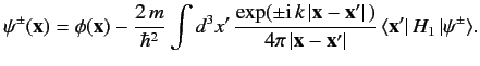
\ref{919} \ref{920} 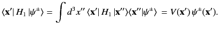
\ref{921} 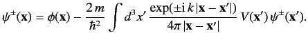
\ref{922} \( \langle {\bf x} \vert {\bf k}\rangle = \frac{ \exp(\,{\rm i}\,{\bf k}\cdot{\bf x}) }{(2\pi)^{3/2}}.\) \ref{923} ![$ \langle {\bf k}\vert{\bf k}'\rangle =\int d^3 x\, \langle {\bf k}...
...\, {\bf x}\cdot({\bf k} -{\bf k}')]} {(2\pi )^3} = \delta ({\bf k} - {\bf k'}).$](http://farside.ph.utexas.edu/teaching/qm/lectures/img2159.png)
\ref{924} , where\( r'/r\) and \( {\bf k}' = k\,{\bf e}_r.\) \( r=\vert{\bf x}\vert\) \ref{927} \ref{928} 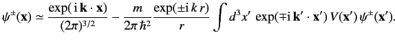
\ref{929} \ref{930} 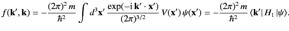
\ref{931} \ref{932} \( {\bf j}_{\rm inc} = \frac{\hbar}{(2\pi)^{3}\,m} \,{\bf k}.\) \ref{934} \( {\bf j}_{\rm sca}=\frac{\hbar}{(2\pi)^{3}\,m} \frac{\vert f( {\bf k}', {\bf k})\vert^{\,2}}{r^2} \, k\, {\bf e}_r.\) \ref{936} \( \frac{d\sigma}{d {\mit\Omega}} = \vert f({\bf k}', {\bf k})\vert^{\,2}.\) \ref{938} Contributors