6.3: Standard Candle

What Do You Think: Brightness

Standard Candles and the Inverse Square Law

Recall flux is a measure of the apparent amount of energy from an astronomical object and luminosity is a measure of the object's true total power output. When you look at a distant streetlight at night, how do you know how bright it really is? It could be an extremely bright light shining at a great distance, or it could be a dim light that is much closer. How are you to know which is the case? Your experience might tell you that all streetlights have roughly the same brightness. Under this assumption, when you see a dim streetlight you have an intuitive sense that it appears dimmer because it is far away (Figure 6.11). But by how much? In the next activity, we will explore the relationship between distance and brightness (Figure 6.11).

Figure 6.11: Streetlights that are farther away look dimmer. Since all streetlights are roughly the same brightness inherently (same luminosity), we know that the dimmer-looking ones only look dimmer because of their distance. Credit: NASA/SSU/Aurore Simonnet

Flux Vs. Distance

In the following activity, you will collect the flux of light around a star by surrounding the star with spheres of ever-increasing size to determine how much lower the flux becomes with distance.

Play Activity

1.

2.

3.

4.

5.

The mathematical expression relating the flux of an object to its distance is known as the inverse square law.

\[F=\dfrac{L}{4\pi d^2}\nonumber\]

In this expression, \(d\) is the distance to an object, \(F\) is its flux (also known as apparent brightness, or intensity), and \(L\) is its luminosity (absolute or intrinsic brightness). This means if an object moves twice as far away, it will look four times dimmer than it did originally. If it moves three times farther away, it will look nine times dimmer, etc. This is illustrated in Animated Figure 6.12.

Play Animation

Animated Figure 6.12: As the lightbulb moves farther away, its apparent brightness decreases by the square of the distance. Here, the size of the bulb is used as a proxy for brightness. Credit: NASA/SSU/Kevin John

The SI units for luminosity are watts, and the units for flux are watts/m², which makes sense because the units for distance are meters. Because of the large numbers involved with astronomical luminosity, sometimes it is expressed in terms of the Sun’s luminosity, which is 4 × 10²⁶ watts, much brighter than a lightbulb! So, if something is “1 solar luminosity,” it is 4 × 10²⁶ watts.

With our detectors, we can measure an object’s flux, that is, how bright it appears. The flux is related to its intrinsic brightness and its distance through the inverse square law. The standard candle technique employs the inverse square law to calculate the distance to an object of known luminosity. The key to using the standard candle method is finding similar objects that all have the same luminosity (or at least known luminosities), so that if we know what type of object we are looking at, we can just look up its luminosity, measure its flux, and use the inverse square law to deduce its distance. The search for standard candles in astronomy is a bit like looking for objects that have the equivalent of a lightbulb’s wattage stamped on them.

Understanding the Inverse Square Law

1.

2.

3.

USE GRAPH

For more practice, answer the following questions below. Star A and Star B have the same luminosity.

• Saying that something is a fraction as bright is the same thing as saying it is dimmer. For example, if something is 10 times dimmer, it is 1/10th as bright.
• Saying that something is a fraction as far is the same thing as saying it is closer. For example, if something is 10 times closer, it is 1/10th as far.

You can choose to state things either way (choose bright or dim, far or close below) as long as you are clear about your choice.

4.

5.

6.

7.

8.

Using the Inverse Square Law

The inverse square law is a very powerful tool used by astronomers to calculate distances to objects that they observe. The inverse square law equation is written as below.

\[ F= \dfrac{L}{4\pi d^2}\nonumber \]

Here we say that \(F\) is the flux (also known as the observed or apparent brightness), measured in watts/m²; \(L\) is the luminosity (also called the intrinsic brightness), measured in watts; and \(d\) is the distance to the object, measured in meters. However, for astronomical distances, meters might not be a very convenient or intuitive unit, so remember that 1 light-year = 9.46 × 10¹⁵ meters and 1 parsec = 3.26 light-years.

1.

2.

Standard Candles

Standard candles have known intrinsic luminosities. Typical Type Ia supernovae can be used as standard candles because they all have intrinsic luminosities that are about 10⁴⁴ W at the peak.

In this activity, we are going to compare four “target” supernovae to a “reference” supernova to determine how much farther away the target supernovae are compared to the reference supernova.

The reference supernova is assumed to have a flux of 100 W/m². The four target supernovae have fluxes that are lower than the reference supernova and are therefore farther away. To determine how much farther away the target supernovae are:

• Move the mouse over each supernova to reveal its flux.
• Compare this flux to the baseline of 100 W/m².
• Use the ratio of the two fluxes to determine the relative distance compared to the “reference” supernova distance according to:
  Relative distance = (100/observed supernova flux)^1/2
• Choose the correct answer for each supernova. When done, press “submit” to check your answers.

Play Activity

Some of the specific objects and relationships astronomers have used as “standard candles” include: spectrally classified stars on the stellar main sequences, certain types of variable stars, the relationship between a galaxy’s rotation speed and its luminosity, and type Ia supernovae. We will discuss each of these in turn below.

Most of the examples we will use in the next sections will describe the luminosities in terms of magnitudes. If you have not read Going Further 3.6: The Magnitude System, now would be a good time to do so.

Spectral Classification and Stellar Main Sequences

An important rung of the distance ladder, called main sequence matching (or main sequence fitting), depends on a comparison of the main sequence for one star cluster to that of another. This provides a relative distance between the two clusters, but not an absolute distance. If the absolute distance to one of the clusters is already known through some other means (such as the moving cluster method described in Section 6.2), then the absolute distance to the other cluster can be found through this comparison.

From our discussion of Planck or blackbody radiation, we expect a hotter star to have a higher luminosity for a given size. This is because, for a blackbody, the emitted radiation is proportional to temperature to the fourth power (\(F\propto T^4\)). We also expect a bigger star to have a higher luminosity, simply because there is more surface area radiating. However, main sequence stars of a given spectral class are nearly the same size. Observationally, we do find that for many stars there is a simple relationship between temperature and luminosity. All main sequence stars of a particular spectral class (which is related to their surface temperature in most cases) have about the same intrinsic luminosity.

Therefore, if we see a main sequence star of a certain spectral type whose distance we wish to measure, we can assume that it has nearly the same luminosity as a nearby main sequence star of the same spectral type. Then we can observe its flux and calculate its distance using the inverse square law. The method works for distances out to tens of thousands of light-years. That is about 10 times farther than the parallax method. However, our ability to use the method still relies on first using parallax on nearby stars to determine the specific relationship between spectral class and luminosity - to calibrate it, in other words.

One challenge to using the spectral type of a star to measure its distance is that astronomers cannot always tell if a star is on the main sequence or not. But there is a foolproof way to get around this problem: compare the main sequences of star clusters. We know that for clusters, the main sequence will stand out in a Hertzsprung-Russell diagram. So plotting the stars in a cluster in a graph of temperature (spectral type) vs. apparent brightness will make the main sequence stars obvious. They can then be compared to a standard HR diagram to determine the distance to the cluster.

Main Sequence Matching for Clusters of Different Distances

This activity shows the main sequences of two star clusters in a Hertzsprung-Russell diagram. Along the horizontal axis is the spectral class, and along the vertical axis is brightness. In the exercise, brightness is given in terms of apparent magnitude. Because all main sequence stars of a given spectral class have the same brightness, the only reason that these two clusters do not lie on top of each other is because they lie at different distances from us. Your job is to slide the lower one up and down until it is superimposed over the upper one. The offset in magnitude will provide a magnitude difference between the two clusters, and this difference can be turned into a difference in distance by using the inverse square law.

The top cluster (shown in blue) is the Hyades, and we have already mentioned that its distance is known from precise Hipparcos satellite parallax measurements. The distance is 46 pc. The other cluster (shown in yellow) lies below the Hyades in the figure. Recall, the greater the apparent magnitude, the fainter the object is.

Play Activity

1.

2.

Use the slider button on the right to slide the cluster main sequence up and down until you have lined it up as best you can with the main sequence of the Hyades cluster. You can read out the difference in magnitudes and the distance on the right. Record these below.

Be careful to use the right side of the main sequence to do the matching and ignore the left side. On the left is where the more massive stars are evolving off the main sequence to become giants, so the matching technique is not valid there. Also, note that you can tell that the Hyades is slightly older than the other cluster because its main sequence turn-off point has moved to lower-mass, longer-lived stars.

3.

4.

This method can be used to determine the distance to any cluster by comparison to the Hyades. All that is required is to create a Hertzsprung-Russell diagram like these, with apparent magnitudes plotted instead of absolute magnitudes.

By matching the main sequences of star clusters, we can compare objects within the disk of our Galaxy to those out into its halo. This is fortunate. Halo objects are much too distant for ground-based parallax measurements. Space-based parallax observations are removing this limitation for halo objects.

Cepheid Variable Stars

Cepheids are a class of extremely bright variable stars. Their luminosity is related to the period of their pulsations: longer-period stars are brighter than shorter-period ones. They are named after the star δ-Cephei (delta Cephei) in the constellation of Cepheus, the first identified example of this particular type of variable star. δ-Cephei can be seen with the naked eye.

This method can be used to measure distances out to about 100 million light-years. Until some Cepheid stars were found close enough to measure their distances using other methods—geometrical methods and main sequence fitting were used historically—Cepheids gave only relative distances. The distances used to calibrate Cepheid luminosities had large uncertainties at first, and these led to large uncertainties in derived distances from Cepheids. Interestingly, the period–luminosity relation for Cepheids was discovered without knowing either their distances or their luminosities.

In 1912, the astronomer Henrietta Leavitt (1868–1921, Figure 6.13), working at the Harvard College Observatory, discovered 20 Cepheid variable stars in the Small Magellanic Cloud (SMC), a small satellite galaxy of the Milky Way. Leavitt knew they were Cepheids because of their distinctive light curves, which make them easy to distinguish from other kinds of variable stars. They display a rapid rise to maximum brightness, and then a more gradual decline (Figure 6.14).

Figure 6.13: American astronomer Henrietta Leavitt at the Harvard College Observatory. Credit: American Institute of Physics

Figure 6.14: Typical Cepheid light curve. A light curve is a graph of brightness vs. time. The light curve for a Cepheid variable star has a characteristic shape, with the brightness rising sharply and then falling off much more gently. The amplitude of the variations is typically 1–2 magnitudes. The period is the time between successive peaks (or troughs) in the curve. Credit: NASA/SSU/Aurore Simonnet

The variations in distance to the individual Cepheid variable stars in the SMC are negligible compared with the much larger distance to the SMC. Essentially, to a good approximation, the stars are all at the same distance. This means that the apparently brightest stars in this group are also intrinsically the brightest. Henrietta Leavitt noticed that the period of a Cepheid variable in the SMC is proportional to its average brightness: brighter Cepheids pulsate with longer periods. This is called the period–luminosity relation for Cepheids. The relation is sometimes also called the Leavitt Relation or Leavitt Law, to honor its discoverer.

By measuring the period of any Cepheid, one can deduce its intrinsic brightness from the Leavitt period–luminosity relation. Then, by measuring the star's apparent brightness, one can calculate its distance using the inverse-square law. This simple procedure makes Cepheid variable stars one of the most important standard candles in the Universe. Not only are they useful distance indicators themselves, they can also be used to calibrate other distance indicators.

Unfortunately, no Cepheids are close enough to allow for an accurate parallax measurement from the ground. To calibrate the Cepheid period–luminosity relation historically, a different calibration, based upon the distances to star clusters, had to be used. The first step was to determine the distance to the Hyades, as we have already discussed. But the Hyades cluster contains no Cepheids, so more distant clusters that did contain Cepheids were compared to the Hyades via main sequence matching. This allowed an absolute calibration for Cepheids to be determined, and this finally allowed an absolute distance for the SMC to be determined. (The actual means by which Cepheids were calibrated was more complicated than this. It had many independent branches, but the distance to the Hyades played an important role for most of them. We are leaving out some of the details for brevity’s sake.)

We have now taken several steps up the cosmic distance ladder, and just as with an actual ladder, each successive step has relied on previous steps. Hopefully, you have begun to understand how astronomical distance measurements somewhat resemble climbing a ladder, where each successive step depends on the previous ones.

Thus far, we have moved from Solar System distances out into the Milky Way, and then to “nearby” galaxies. As we look at the last few rungs of the ladder, we will see how they allow us to measure distances farther and farther across the visible universe.

One of the main scientific reasons for building the Hubble Space Telescope (HST) was to measure the distances to galaxies in the Virgo cluster of galaxies. This project was known as the HST Key Project. The measurements relied on observations of Cepheid variables located in Virgo galaxies. Atmospheric distortions combined with the great distance to Virgo prevent astronomers from measuring Virgo’s Cepheids from the ground. A telescope in space overcomes this problem.

The Virgo Cluster contains some 2,500 galaxies, among them the spiral Messier 100 (Figure 6.15). From repeated observations of M100, astronomers were able to identify more than a dozen Cepheid variables and measure their brightness as a function of time. From the Hubble measurements of Cepheid variables in M100, the periods of the variables, and hence, their intrinsic luminosities could be determined (see Figures 6.16 and 6.17). Once both the intrinsic and apparent brightnesses were known, the distance to M100 could be calculated. Such observations of M100 and other galaxies in Virgo enabled astronomers to calibrate the period–luminosity relation to higher precision than had been possible in the past. In turn, it allowed calibration of distance measurement techniques suitable for larger distances than with Cepheids alone.

Figure 6.15: The spiral galaxy Messier 100, as imaged by the Hubble Space Telescope. Credit: NASA/STScI

Figure 6.16: Hubble Space Telescope tracks down Cepheid variable stars in M100. Hubble’s high-resolution camera detected and picked out one of the Cepheid variable stars used in the next activity. The star is located in a star-forming region in one of the galaxy’s spiral arms (the star is at the center of the box). Credit: ESA/ESO

Figure 6.17: Six images taken at different times depicting one of the Cepheid variable stars in the galaxy M100 are shown. The Cepheid is in the center of each frame. It is clear that the Cepheid varies in brightness over time. Credit: ESA/ESO

Measuring the Distance to M100 Using Cepheids

In this activity, we will measure the distance to M100 using Cepheids, retracing the steps of the HST Key Project Team.

A. The Period-Luminosity Relation for Cepheids

The relation between a Cepheid’s period (the time over which its brightness varies) and its absolute magnitude (a measure of its luminosity) is given by the following expression:

\[M=−2.8log(P)–1.4\]

where \(M\) is the absolute magnitude, log is the base 10 logarithm, and P is the period in days.

This expression is shown in graphical form in the following figure:

Absolute magnitude (plotted along the vertical axis) vs. period in days (running along the horizontal axis) for Classical Cepheid stars is shown by the red curve. This is the Leavitt Period-Luminosity relation from above shown in graphical form.

1.

2.

B. You will now examine Cepheid light curves from HST. (Credit: Ferrarese et al., 1996, ApJ, 464, 568.)

1. From the light curves, determine the periods of five Cepheids and enter the periods that you measured into the data table. The period is the time between successive peaks (or troughs) of the light curve. Click on the curves to read the data. Enter the period into the data table below in section D.

2. Determine the absolute magnitude M of each Cepheid from the period using either the graph above or the expression in part A, and enter it into the data table below in section D.

C. The Inverse Square Law: Absolute and Apparent Magnitude

The absolute magnitude of a star corresponds to the luminosity of a star (related to its inherent brightness), and the apparent magnitude corresponds to the flux (related to how bright it appears to you). If a star is very far away from you, it will appear dim even if it is a very bright star. Thus, the difference between the absolute magnitude and the apparent magnitude is related to the distance. The relation can be written mathematically as:

\[d=10^{(m−M+5)/5}\]

where \(d\) is the distance in parsecs, m is the average apparent magnitude and M is the absolute magnitude. This relation can be derived from the inverse square law. This expression is shown in graphical form in the following figure.

The figure above shows the distance vs distance modulus, m-M, relation. It has a linear axis for distance modulus and a logarithmic axis for distance. To use the figure, find the appropriate value of distance modulus along the horizontal axis, then scan directly upward until you intercept either the green, blue or red line. Where the line meets your chosen distance modulus you can read the corresponding distance by scanning horizontally over to find the value for distance on the vertical axis: The green line gives the distance in parsecs, the blue line gives it in kiloparsecs and the red line gives the distance in megaparsecs. In the areas where the lines overlap, you can use either unit. For example, for a distance modulus m-M=20, the figure shows that the distance is 100 kiloparsecs (where the blue line intersects m-M=20) or, if you prefer, 0.1 megaparsecs; this is where the red line intersects m-M=20. These are the same distance expressed in different units, and you can use whichever unit you like. This unusual way of plotting the relation allows us to more easily see distances corresponding to a wide range of distance modulus.

1. The average apparent magnitude is halfway between the maximum and minimum brightness in the light curve. Measure the average apparent magnitude m for each Cepheid that you previously studied in part B. Enter your results in the data table in section D.

2. Using the values of the absolute and apparent magnitude for each Cepheid, determine its distance d. Enter your results in the data table in section D.

D. Data Table

E. Discussion

1.

2.

3.

Tully-Fisher Relation

The luminosity (\(L\)) of a spiral galaxy is proportional to its rotational velocity (v) to the fourth power:

\[ L\propto v^4 \nonumber \]

The relationship is called the Tully-Fisher relation. By using spectral lines, we can easily determine the rotational velocity, and hence, the luminosity of a galaxy. A similar relation, called the Faber-Jackson relation, holds for the characteristic velocities of the stars in elliptical galaxies and is also measured from the galaxies’ spectra. These methods work for greater distances than methods based on stars because galaxies are much brighter than stars and can be seen to much greater distances than can individual stars. In practice, the Tully-Fisher and Faber-Jackson relations can be used out as far as we can measure the spectral lines of a galaxy. This is out to billions of light-years.

The relationship between stellar orbital speed and brightness becomes apparent when astronomers study galaxies in a given galaxy cluster. The galaxies in a cluster are essentially all at the same distance, and so this is reminiscent of how Henrietta Leavitt observed Cepheids in the Small Magellanic Cloud to discover the period–luminosity relation. Without a nearby calibration, only relative distances can be determined, not absolute distances. The HST Key Project for Cepheids in the Virgo Cluster of galaxies provided a precise local calibrator for the Tully-Fisher and Faber-Jackson relations.

Tully-Fisher Relation

In this activity, you will study the Tully-Fisher relationship between rotational velocity and intrinsic brightness for a set of spiral galaxies. The method will bear some similarities to the Cepheid distance method in that there is a relationship between luminosity of an object and an easily measurable quantity. In the case of Cepheids, the relationship is between luminosity and period of pulsations. For spiral galaxies, the relationship is between luminosity and rotation speed of the galaxy.

The rotation speed of a galaxy is determined from its spectrum, specifically the 21-cm emission line from neutral hydrogen gas. If a galaxy is rotating, the gas in the part of the galaxy rotating toward us will show a blueshift, while the gas in the part of the galaxy rotating away from us will show a redshift. However, this motion is superimposed on the net motion of the galaxy in space. This motion is almost always much larger than the rotation speed of the galaxy, and it is away from us for all but a few galaxies. So the net effect is that the entire emission line will be redshifted, but the parts rotating away will have a larger redshift than the parts moving toward us. The center of the galaxy will not be rotating toward or away from us.

The emission line from hydrogen in a galaxy looks strange. That is because the entire galaxy contains hydrogen and the entire galaxy is rotating. We see different components of that rotation depending on where we look. For instance, the outer parts are moving almost straight toward us or straight away from us, so we see the entire motion reflected in the redshift there. But if we look toward the center of the galaxy, we see a lot of gas that is traveling across our line of sight, and only a little that is moving toward or away. This effect causes the emission line to be smeared out in a broad plateau. It is the width of this plateau that gives us the rotation speed of the galaxy.

Play Activity

A. Determining the Tully-Fisher Relation

In the first part of this activity, 10 galaxy spectra are available. You should use at least six of them in order to obtain a good determination of the Tully-Fisher Relation.

1.

2.

3.

B. Using the Tully-Fisher Relation to Estimate the Distance to Galaxies

In this part of the activity, you will use the Tully-Fisher Relation that you created in Part A to determine the distances to three additional galaxies.

1.

This is the general way that the Tully-Fisher relation is used to measure the distances to galaxies. We have omitted some of the complicating details so that you get a better understanding of how the method works.

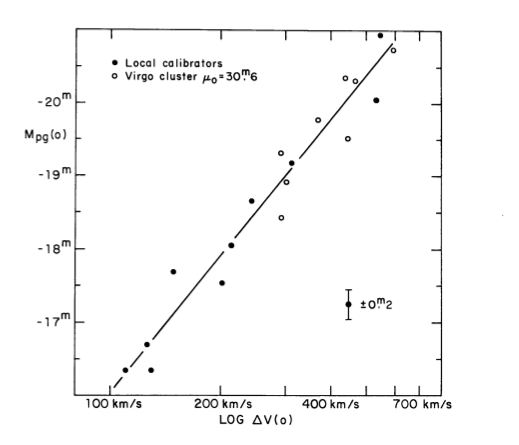
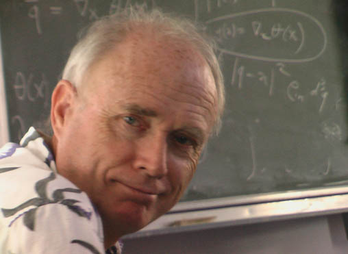
Now that you have done the Tully-Fisher activity, you may be interested in seeing the original data (Figure 6.18), published in 1977. R.B. Tully and J.R. Fisher are shown in Figure 6.19.

Figure 6.18 The original data published by Tully and Fisher in 1977. The plot shows the photographic magnitude of the galaxy plotted vs. the rotation speed. Credit: Tully, R.B. and Fisher, J.R. 1977, Astronomy and Astrophysics, 54,3, 661

Figure 6.19: (a) R. Brent Tully and (b) J. Richard Fisher today. R. Brent Tully is an astrophysicist at the Institute for Astronomy in Hawaii. He went to graduate school at the University of Maryland before moving to Hawaii, one of the world’s best places to do astronomical observations at visible wavelengths. J. Richard Fisher is a radio astronomer, working at the National Radio Astronomy Observatory in Charlottesville, Virginia. Dr. Fisher also went to graduate school at the University of Maryland and is an adjunct professor at the University of Virginia. Credits: (a) www.ifa.hawaii.edu/~tully/ (b) www.astro.virginia.edu/people//faculty/jrf2v/

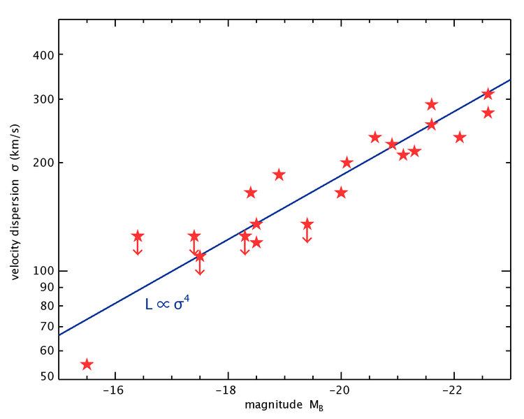
The Faber-Jackson relation (Figure 6.20) was developed in 1976 by astronomers Sandra Faber (Figure 6.21) and Robert E. Jackson. It relates the luminosity of an elliptical galaxy to the spread in velocities observed near the galaxy’s center.

Figure 6.20: Data used in the original Faber-Jackson relation. The plot shows the velocity dispersion vs. the galaxy’s brightness in magnitudes. Credit: Faber, S.M. and Jackson, R.E. 1976, Astrophysical Journal, 204,668

Figure 6.21: Sandra Faber is a professor at the University of California, Santa Cruz, and is a prominent cosmologist who has won many awards for her work, including the Heineman Prize, the Harvard Centennial Medal, and the Franklin Institute’s Bower Award. She is a member of the National Academy of Sciences and was an early leader in the use of the Hubble Space Telescope for cosmological observations. Robert E. Jackson was Faber’s graduate research assistant at UC Santa Cruz, and he helped analyze the data that led to the determination of the relation. Credit: http://astro.ucsc.edu/~dept/faculty/faber.html

Type Ia Supernovae

The shape of the light curve of certain supernovae is related to their luminosity. These supernovae, designated as type Ia, are the result of the thermonuclear explosion of a white dwarf star. This distance method works out to a few billion light-years because the supernovae are so bright that they can be seen at large distances. Supernova distances can be calibrated with the Tully-Fisher and Faber-Jackson relations. Because supernovae are quite rare, we do not have examples in galaxies that are close enough to allow the use of Cepheids for distance calibration. The top panel in Figure 6.22 shows the light curves from many type Ia supernovae, while the bottom panel shows the same supernovae corrected to have the same absolute brightness and decay time. This illustrates how these supernovae can be used as standard candles. A light curve, as we discussed in section 6.3.3, is a plot of brightness vs. time.

Figure 6.22: The top panel shows the light curves (light emitted as a function of time) of many different type Ia supernovae, which have occurred at different distances. The bottom panel shows how these supernovae can be used as standard candles once their light curves have been corrected by the “stretch-factor.” Credit: Courtesy of Alex Kim and the Supernova Cosmology Project

When a star explodes as a supernova, its brightness rises very rapidly, increasing in about three weeks until it rivals the brightness of the galaxy in which it is located. The brightness then begins to turn over, and the star slowly fades over many weeks or months. In the case of Type Ia supernovae, the peak brightness reached is nearly the same for all of them. This is not true for other types of supernovae.

During the 1980s and 1990s, astronomers studying supernovae found that light curves for this kind of supernova had a very useful property. The dimmer the peak brightness of the supernova, the faster it dropped in brightness in the weeks following the peak. In fact, astronomers found a simple linear relationship between the absolute magnitude of a type Ia supernova and its drop in magnitude in the first 15 days after its maximum brightness. This relationship is called the Δm₁₅(B) relationship, with B indicating that the measurement is to be made using the B (blue) filter on the telescope and camera.

The reason this relationship is so useful is that it allows a simple timing measurement to be converted into a brightness measurement, and thus, for type Ia supernovae to be used as standard candles. This should be familiar to you from your study of Cepheid variables.

Examples of supernova light curves are shown in Figure 6.23. The left-hand panel shows the light curves of five supernovae, with absolute magnitude being plotted vs. time—these supernovae occurred in galaxies of known distance, so their absolute magnitudes could be determined from their apparent magnitude and the distance to the galaxy. The right-hand panel shows the same supernovae, but they have been shifted such that their peak brightness coincides. Some of these curves decrease in brightness more quickly than others. But much more interesting, if you compare the two plots, you will see that the faster the drop from peak brightness, the dimmer the supernova. Furthermore, after about 20 days, all of the light curves drop at the same rate, so it is this initial drop from peak brightness that is important for determining the absolute magnitude of the supernovae. There is a linear relationship that gives the peak absolute brightness in terms of the decrease in brightness over the first 15 days after maximum, Δm₁₅(B):

\[M_B=−0.748[\Delta m_{15}(B)−1.1]−19.258 \nonumber \]

In this equation, \(M_B\) is the absolute magnitude in the \(B\) (blue) filter.

Figure 6.23: Light curves from five selected type Ia supernovae. The left-hand panel shows the absolute brightness for each supernova as a function of time. The right-hand panel shows the results when the light curves are adjusted to have the same value for peak brightness. Note that the dimmer supernovae in the left-hand panel fall faster in the right-hand panel. Credit: NASA/SSU/Aurore Simonnet

Supernovae Type Ia and Distances

In this activity, you will use the relationship between the peak absolute brightness and the decrease in brightness over the first 15 days after maximum to determine the absolute brightness for several supernovae. You will then estimate the distances using the relationship between absolute brightness and the apparent brightness.

Play Activity

1. Plot the light curve for the first supernova, SN 1991T, by clicking on the button labeled with its name. Brightnesses are given in magnitudes and the values for the points can be found by moving your mouse over them.

2. Now click the Calculate Magnitude button. You will see the equation for the absolute magnitude, MB, displayed. Click the “equals” button to compute and display the absolute magnitude. Record it in the data table.

3. Now click on the Calculate Distance button. The expression for the distance to the supernova will display. This will not look like the inverse square law for light, but it is. Recall that we are measuring brightness in magnitudes, and that those are related to the log of the true brightness. That is why the formula might not look the way you expect. It will be filled in with the correct absolute magnitude, which you have just calculated, and the corresponding apparent magnitude, which is read from the point you chose as the peak brightness of the light curve. Hit the “equals” button to display the distance in Mpc. Record the distance in the data table.

4.

5.

6.

7.

This activity outlines the basics of how astronomers use supernovae to determine the distances to galaxies. Only galaxies with a supernova observed in them can be measured this way, but even distant galaxies can be measured because type Ia supernovae are so bright. Supernovae are rare, but there are many, many galaxies in the distant universe. As a result, the type Ia supernova distance method has been extremely useful for building our understanding of the evolution of the Universe. We will return to this topic again when we study the cosmic expansion of the Universe in later chapters.