6.5: Wrapping It Up 6 - The Supernova of 1885

In the year 1885, what was thought to be a bright nova (“new star”) was observed in the center of M31, now known to be the Milky Way Galaxy’s closest large galactic neighbor, the Andromeda Galaxy. The nova was originally called S Andromedae (S And for short), using the letter-constellation naming scheme commonly employed for variable stars, of which novae are one class. At the time, the distance to M31 was unknown, so the true brightness of this object was also not known to astronomers of the day. Since that time, we have learned that M31 is actually quite distant, and that the object observed in 1885 was not a nova, but what we now call a supernova—an exploding star, millions of times brighter than the much more common novae.

In the months after its discovery, S And gradually faded from view. However, more than a century later, two American astronomers, Robert Fesen of Dartmouth University and Andrew Hamilton of the University of Colorado, managed to obtain an image of the supernova remnant using the 4-meter telescope at Kitt Peak Observatory in Arizona. This image was followed up with much more detailed images using the Hubble Space Telescope. In addition, the pair was able to measure an absorption spectrum from the remnant, also using Hubble. In this activity, you will use the data acquired with the Hubble Space Telescope to measure the distance to the supernova remnant, and hence, to the center of the nearby galaxy, M31, in Andromeda.

Figure A.6.4: This image shows the center of the galaxy M31. The dark inset is an image of the core, and the orange circle to the lower right is SN 1885a. Credit: Courtesy of Andrew Hamilton, CU Boulder.

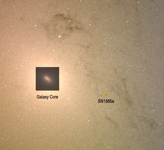
If you examine the Hubble image of the core of M31 (see Figure A.6.4), you will notice a faint circle to the right of and below the bright nucleus of the galaxy that appears darker than the surrounding regions. The circle appears quite small. That is the supernova remnant of S And, the star that was seen to explode in 1885, today known as SN 1885a. The remnant appears darker because it is composed of an expanding cloud of cold gas. It absorbs and scatters light emitted from behind it, just as thick clouds of dust or water vapor in Earth’s atmosphere absorb and scatter light from the Sun, making them appear darker than the surrounding sky from our vantage on the ground.

To measure the distance, you will use the following procedure:

1. Use the image to measure the angular size of the remnant.
2. Use the spectrum to estimate the expansion velocity of the cloud.
3. Use the age of the remnant and its expansion velocity to determine the physical size of the cloud.
4. Use the small-angle formula to determine a distance from the angular size and physical size.

Play Activity

Part I: Measuring the Angular Size of the Supernova Remnant

Click the "Next" button.

An expanded version of the HST image of the supernova remnant is provided. The scale has been increased so that you can see the individual pixels of the image. Each of these pixels is about 0.049 arcseconds across.

1.

Part II: Measuring the Expansion Velocity of the Remnant

Click “next step.”

In this part, you will use the Spectral Analysis tool to examine the absorption spectrum of the supernova remnant. You will notice two prominent absorption features. Line 1, which is the large feature in the center, is mostly caused by Ca II (singly ionized calcium), with a small contribution from Fe I (neutral iron). The one on the right is due to Fe I (neutral iron). Atoms emit or absorb narrow lines in the electromagnetic spectrum when their electrons change from one energy level to another. But the lines in this spectrum are not narrow; they are quite broad.

The lines in this spectrum are broadened by the motion of the absorbing gas. The supernova remnant can be modeled as a spherical cloud of expanding material ejected when the star exploded. The gas on the near side (closest to us) is expanding toward us. Since it is moving toward us, its absorption line is shifted to the blue from our viewpoint. On the other hand, the gas on the far side of the remnant is moving away from us, so its absorption lines are shifted to the red. Since the remnant is composed of gas moving directly toward us, directly away from us, and at all intermediate velocities, we see the intrinsically narrow absorption lines broadened into the features in the spectrum. By using the amount of broadening and the Doppler formula, we can estimate how fast the gas is moving.

By fitting a special kind of curve, called a Gaussian (popularly known as a bell curve), over the data, we can determine the width of the absorption lines, and hence, the expansion rate of the supernova. It is not important that you understand the details of a Gaussian curve, as those are incorporated into the Spectral Analysis tool. All you have to do is use your mouse to fit a Gaussian on each of the absorption features in turn.

To use the Spectral Analysis tool:

• Click and drag the left button to move the tool into place.
• Click and drag the right button to change the width of the curve.
• Click and drag the slider to change the depth of the curve.

1.

2. Repeat for line 2.

3.

Part III: Determining the Physical Size of the Remnant

The physical size of the supernova remnant can be calculated by multiplying the expansion rate by its age, assuming the expansion speed has remained constant. It is also necessary for you to know that the image you are using was taken by the Hubble Space Telescope in 1998.

1.

2.

Part IV: Determining the Distance to the Remnant

Using the size you just determined, along with the angular size you measured from the image, you will now determine the distance to S And by employing the small-angle approximation.

1.

2.

3.