8.1: Making Models for Rotation

Learning Objectives

• You will be able to use multiple representations to understand a velocity distribution (words, graphs, pictures, equations).
• You will be able to use multiple representations (words, graphs, pictures, equations) to understand an everyday example of a system with a velocity distribution that is constant with radius.
• You will be able to use multiple representations (words, graphs, pictures, equations) to understand everyday examples of systems with velocity distributions that are inversely proportional to radius.

What Do You Think: Models

In this chapter, we will talk a lot about models. Not the kind of models you might have made as a child, of planes or boats or cars. The models we will talk about will be conceptual models. They will involve mathematics and physics. In the dialogue above, models of galaxies are mentioned. What other models can you think of that we use in everyday life? Try to think of several common examples of conceptual and physical models that are commonly used.

This section of the chapter will be focused on using models to describe the velocities of objects as they rotate. Later, we will use models to describe how mass is distributed in objects. We will link our models for mass and velocity using the physics of gravity. Later still, we will compare models to better understand the motions of stars and gas in galaxies, and the motions of galaxies in galaxy clusters. Then we will explore the constituents of the mass of galaxies and galaxy clusters. As you might have guessed from the title of this chapter, dark matter will play a large role in the discussions in this chapter.

Rotation of a Rigid Disk

When we think of rotating objects, some of the first things that come to mind are wheels spinning about their axles, or (if you are old enough) records or CDs. Many objects in nature rotate this way. Because these examples are solid, disk-shaped objects, we will call them rigid disks in this chapter.

We can take a closer look at the example of a wheel. More specifically, look at how the solid material that makes up a wheel rotates about its axle. Suppose the wheel rotates once per second, or in other words, it rotates with a frequency of 1 Hz. A point on the wheel that is close to the axle will go around once each second, and a point on the wheel that is close to the outer edge will also go around once each second. Any point on the wheel makes one full rotation each second.

Now think about the velocities of three different points on the wheel (Figure \(\PageIndex{1}\)). Point A, toward the center of the wheel, will go around a small circle each second. Point B, which is farther out from the center than Point A, will go around a larger circle each second. Point C, on the outer edge of the wheel, will go around an even larger circle each second.

Figure \(\PageIndex{1}\): Rotation of points on a wheel. Points A, B, and C on this wheel all go around a circle in the same amount of time. However, since they are at different distances from the center of the wheel, the sizes of the circles they travel around are different, and so their velocities are different. Credit: NASA/SSU/Aurore Simonnet

Example: Velocities at Different Points on a Rigid Disk

Let’s calculate the velocity of Point A on the wheel. Suppose that Point A is 2 m from the center of the wheel and the wheel is rotating with a frequency of 1 Hz.

• Given: radius \(r = 2 m\), \(f = 1 Hz\)
• Find: velocity \(v\)
• Concepts: We can get the velocity from: velocity = distance / time

The size of the circle that Point A will travel around can be calculated using the formula for circumference:

\[C = 2πr \nonumber \]

And if the frequency is 1 Hz, the time to travel once around is 1 second.

Solve

The distance Point A will travel in one second is

\[C = (2)(π)(2 m) = 12.6\, m. \nonumber \]

The time to travel once around is 1 second, so the velocity of Point A is v = 12.6 m / 1 s = 12.6 m/s.

Questions

To understand the motion at various points on the wheel, it can be helpful to graph the rotation curve of the wheel. A rotation curve is a graph of velocity versus radius. We do this because it not only helps us better understand the motion of the wheel, but by comparing the rotation curves of different objects (such as wheels, or even the Solar System and galaxies), we can see whether they rotate in the same way or differently. We can also use some physics to begin to examine why they rotate the way they do.

Rotation Curve of a Rigid Disk (Wheel)

We can use the graphing tool to graph the rotation curve of the wheel described above. We want to plot radius on the x-axis, and velocity on the y axis. We can type the following three data points into the graphing tool (we will ignore units for the time being):

• Point A, \(r = 2\), \(v = 12.6\)
• Point B, \(r = 10\), \(v = 62.8\)
• Point C, \(r = 30\), \(v = 188.5\)

The resulting graph looks like the one in Figure \(\PageIndex{1A}\):. See if you can make a graph like this, using the graphing tool.

Figure \(\PageIndex{1A}\): This graph represents the rotation curve of a wheel. Credit: Sonoma State University

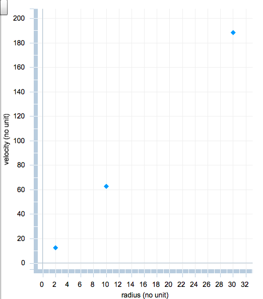
The points on the rotation curve for a rigid disk form a straight line. This tells us that the velocities at different points on the wheel are proportional to their distances from the axle. In other words, as the distance from the center of the wheel gets larger, the velocity of the point on the wheel gets larger. We write this mathematically as

\[v\propto r \nonumber \]

where \(v\) corresponds to velocity, and r corresponds to radius, or distance from the wheel’s axle. In this equation, the Greek symbol ∝ is used to represent proportionality. This relationship between velocity and radius holds for any rigid disk that is rotating about its center. Examples include a CD, the wheel of a bicycle, and an LP record.

Going Further 8.1: Linear and Angular Velocity

Until you do the math, like we have above, it may not seem obvious that a point toward the center of a rotating rigid disk, like a wheel, has a smaller velocity than a point farther from the center of the wheel. Since both points go around a circle in the same amount of time, it seems like they should have the same velocity.

However, as we have calculated, the points have different velocities because they are going around different-sized circles. The inner point goes around a smaller circle, so it travels a smaller distance in the same amount of time that the outer point travels around a larger circle (larger distance).

This is how the calculation works out when we study the linear velocity of the points on the wheel. Linear velocity refers to the linear distance an object has moved (and in what direction) in a given amount of time. This is the kind of velocity we are used to thinking about and have concentrated on so far in these modules:

\[\text{linear velocity}=\dfrac{\text{distance}}{time}=\dfrac{d}{t} \nonumber \]

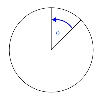
However, physicists also use angular velocity to describe the motion of objects that turn. Angular velocity is defined as the size of the angle an object rotates through in a given amount of time (Figure \(\PageIndex{1B}\))

\[\text{angular velocity}=\dfrac{\text{angle}}{\text{time}}=\dfrac{θ}{t} \nonumber \]

Look at the angular velocities of different points on a rotating wheel—it may help to refer back to Figure \(\PageIndex{1}\). Point A, close to the center of the wheel, Point B, a bit further out, and Point C, toward the edge, all make one rotation in the same amount of time. This means that each point rotates through an angle of 360 degrees (one full circle) in the same amount of time. In other words, all three points have the same angular velocity.

So, if your intuition was telling you earlier that all three points had the same velocity, you were on the right track—they do all have the same angular velocity, and in some cases it is very helpful to study angular velocity. However, for the rest of this chapter, we will continue to focus on studying linear velocity.

Figure \(\PageIndex{1B}\): Angular velocity. This figure shows the angle a disk rotates through as it spins. Credit: Sonoma State University

Swirling Vortex

Not every rotating thing we can think of in our everyday lives rotates like a rigid disk, or wheel. For example, we can think of water swirling toward a drain, or dust devils and tornadoes— though hopefully you are not experiencing too many tornadoes in your everyday life! These sorts of phenomena are called vortices (plural for vortex).

In a vortex such as water swirling toward a drain, the rotation is actually very different than for a rigid disk like a wheel. Usually, the water closest to the drain will make one full rotation in a shorter amount of time than the water farther from the drain. The two movies below compare rigid disk rotation and rotation that is more similar to water swirling down a drain.

Figure \(\PageIndex{2}\): To the left is a movie showing rigid disk rotation, in which a point on a ring makes one rotation in the same amount of time as a point on any other ring. To the right, we see a movie showing rotation like that of water going down a drain. In this case, points on rings closer to the center make one full rotation in a shorter amount of time than points on rings farther from the center. In other words, a point on an inner ring will “lap” a point on an outer ring. Credit: Wikipedia Creative Commons.

There are two types of velocity models that will result in rotation similar to that of water going down a drain, where material closest to the center of rotation will make a full rotation in a shorter amount of time than material farther from the center of rotation. The first type of velocity model we will talk about may seem the most obvious: it is the case where material closer to the center of rotation has a higher velocity than material farther from the drain.

We can look at an example to understand this better. Suppose a physicist is studying the motion of water as it swirls toward the drain in her lab sink. She fills up the sink and drops three floats in the water at different distances from the drain. She then times how long it takes each float to make one circuit around the drain (Figure \(\PageIndex{3}\)).

Figure \(\PageIndex{3}\): In this example of water going down a drain, the floats at points A, B, and C each make one full rotation in different amounts of time. Credit: NASA/SSU/Aurore Simonnet

The physicist hypothesizes that she can describe the motion of the water using the following velocity model:

\[v=\dfrac{0.05 m^2/s}{r} \nonumber \]

where \(v\) is the velocity of the water at a given point in m/s, and r is the radius (or the distance) between that point and the drain, given in meters. Note that in this model, velocity is inversely proportional to radius. In other words, as the distance from the drain increases, the velocity of the water decreases. In the activity below, we will calculate how it would take each float to circle the drain once.

Worked Example: Velocities Decreasing With Increasing Radius

Assume Float A is 0.1 m away from the drain. Using the physicist’s velocity model, what would we expect the velocity of Float A to be as it rotates around the drain?

• Given: \(r = 0.1\, m\)
• Find: \(v\), Float A’s velocity
• Concept: \(v = (0.5\, m^2/s)/r\)
• Solution: \(v = (0.05\, m^2/s)/ (0.10 m)\) or \(v = 0.5 m/s\)

How long would it take the float to circle the drain once?

• Given: \(v = 0.5\, m/s\) and \(r = 0.1\, m\)
• Find: \(t\), the time it takes Float A to circle the drain once (also known as the period)
• Concepts: \(v = d/t\), \(d = 2/πr\)
• Solution: \(d = 2πr = 2π(0.1 m) = 0.628\, m\)
• Using some algebra, we can convert the expression \(v = d / t\) to \( t = d / v\)
• t = (0.628 m) / (0.5 m/s)
• t = 1.26 s

Questions

Rotation Curve of Water Rotating Around Drain

1. Now use the graphing tool to look at the rotation curve that results from the physicist’s model of water rotating around the drain of her lab sink. Use the velocities calculated for Floats A, B, and C in our example, and the distances (radii) of these floats from the drain. Be sure to plot the radii on the x-axis, and the velocities on the y-axis. Describe your graph.

2. Your plot should look like Figure \(\PageIndex{3A}\): below. Note that in the graph, the closer the float is to the drain, the higher is its velocity. The farther the float is from the drain, the lower is its velocity. This is what we expect from the equation the physicist used to model the motion of water in her sink, in which velocity is inversely proportional to radius.

Reconcile any differences between Figure \(\PageIndex{3A}\): and your graph and describe them here.

Figure \(\PageIndex{3A}\): Rotation curve of water rotating around drain. This graph shows the rotation curve that results from a velocity model in which velocity is inversely proportional to radius. Credit: NASA/SSU

Cars Driving Around a Roundabout

There is another, less intuitive velocity model that can result in an object or point toward the center of rotation making a full circle in a shorter amount of time than an object or point farther from the center of rotation (like in the case of water rotating around a drain). This is the case where the velocities at all points, no matter what their distances are from the center, are the same. Imagine that three cars are driving around a roundabout. Each car is in a different lane (Figure \(\PageIndex{4}\)), but they all are traveling at the same speed.

Figure \(\PageIndex{4}\): Cars A, B, and C in this example all have the same velocity. However, they will travel around different-sized circles (depending on their distance from the center of rotation, or which lane they are in). Therefore, it will take each car a different amount of time to go around the roundabout, or make one full rotation. Credit: NASA/SSU/Aurore Simonnet

Mathematically, we can describe the cars’ velocities with a model in which the velocity is a constant number, since each of the cars has the same velocity:

\[v=constant \nonumber \]

In other words, the velocity at any point (in any lane) is the same and does not depend at all on the distance from the center of rotation (the center of the roundabout). We will perform some calculations to see how this velocity model can result in cars at different distances from the center of rotation taking different amounts of time to complete a full circle.

Worked Example: Cars Driving Around Roundabout: Constant Velocity Model

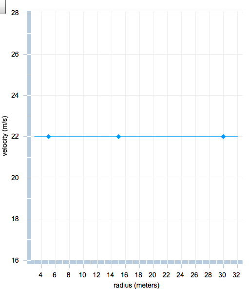
We will describe the cars' motion by a constant velocity model with v = 22 m/s. That means the velocity any car in any lane is 22 m/s, no matter how near or far the car is from the center of the roundabout.

1. Assume Car A is 5 m away from the center of the roundabout. How much time will it take Car A to make one full circle around the roundabout?

• Given: v = 22 m/s and r = 5 m
• Find: t, the time it takes Car A to circle the roundabout once
• Concept: t = d / v, d = 2πr
• Solution: d = 2πr = 2π(f m) = 31.4 m
  → t = (31.4 m) / (22 m/s) = 1.43 s

Questions

At all distances from the center of rotation, the velocity is the same. So the graph looks like a horizontal line (Figure \(\PageIndex{4A}\)). This rotation curve graph may not seem very exciting, but we will see that it can teach us a great deal when we discuss the rotation curves of galaxies!

Figure \(\PageIndex{4A}\): Rotation curve for constant velocity model. This graph shows the rotation curve that results from a constant velocity model (here the velocity is 22 m/s). Credit: Sonoma State University

In this section, we have studied several different mathematical relations between velocity and radius. This next interactive will give you the opportunity to connect the equations that you have studied to an animation created using a simple computerized model.

VELOCITIES AND GRAPHS

Play Simulation

The multi-colored rings on the left-hand side of the activity can be arranged to move at different rates by choosing a rotation curve (X, Y, or Z) from the menu above the graph on the right-hand side. Which rotation curve best describes each of the following situations?