9.4: The Geometry of Special Relativity - Spacetime

Learning Objectives

• You will recall the mathematical concepts of coordinate systems and the Pythagorean theorem.
• You will be able to draw/interpret spacetime diagrams for a variety of scenarios.

What Do You Think: Spacetime

The examples in the previous sections show how space and time are different for different observers depending on their relative motion. One way to understand this concept is to consider the geometry related to special relativity. It has some similarities to the geometry you may have already learned about in school, but it also has some stark differences. The differences result from the fact that the speed of light is the same for all observers, no matter their state of motion. In this section, we will introduce the idea of spacetime and its peculiar geometry.

Geometrical Refresher

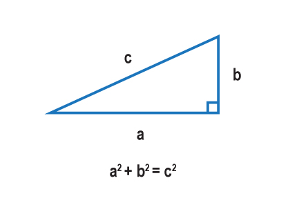
The geometry that most of us learn in school is that of a plane. It is sometimes called plane geometry, or Euclidean geometry after Euclid, the mathematician in Ancient Greece who codified its properties. In plane geometry, we learn that the angles of a triangle must all add up to 180 degrees, parallel lines never meet, and the ratio of the circumference of a circle to its diameter is the number \(\pi\). Another relation that holds true in plane geometry is the Pythagorean theorem , which describes the relation between the three sides of a right triangle. The Pythagorean theorem is illustrated in Figure 9.5 and can be written as:

\[a^2+b^2=c^2 \nonumber \]

where \(a\) and \(b\) are two sides of a right triangle and \(c\) is the longest side, called the hypotenuse. It is the diagonal side in the diagram below.

Figure 9.5: The Pythagorean theorem describes the relationship between sides a, b, and c of the right triangle shown. Credit: NASA/SSU/Aurore Simonnet

When we talk about plane geometry, we often talk about points on a plane and the relationships between them. For instance, in Figure 9.5, three points make the vertices of the triangle. Those points can be described by their (x,y) coordinates in a coordinate system, as shown in Figure 9.6.

Figure 9.6: This is the same right triangle as in the previous figure, now with the (x,y) coordinates of the vertices labeled. The vertices are points A, B, and C. They have coordinates (x_A,y_A), (x_B,y_B), and (x_C,y_C), respectively. The various relationships between coordinates and lengths are also shown. Credit: NASA/SSU/Aurore Simonnet

Once we have chosen a coordinate system, we can write expressions relating points on the plane using those coordinates. So for Figure 9.6, we can use the coordinate system to write expressions for the length of each side of the triangle:

\[a=x_B–x_A \nonumber \]

\[b=y_C–y_B \nonumber \]

\[c^2=(x_B–x_A)^2+(y_C–y_B)^2 \nonumber \]

These expressions are true because the length of the side of the triangle labeled \(a\) is the difference in the \(x\)-coordinates of points A and B. Similarly, the length of side \(b\) is the difference in the \(y\)-coordinates of points B and C. The length of side \(c\) is given by the Pythagorean theorem. In addition, points A and B both have the same \(y\)-coordinate, and points B and C have the same \(x\)-coordinate.

Compare the situation just outlined to the one shown in Figure 9.7. We have not changed the triangle ABC at all. It still has the same sides and the same angles, and it has the same relationships between the points A, B, and C. However, we have rotated the coordinate system we are using to describe the positions of things, and so the coordinates of each point have changed.

Figure 9.7: Same right triangle, but now with slightly rotated coordinates. Credit: NASA/SSU/Aurore Simonnet

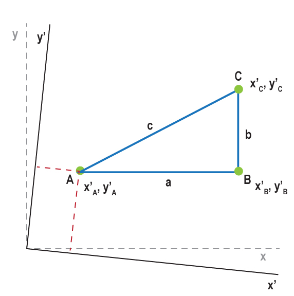
The mathematical expressions for the lengths of the sides a, b, and c in these rotated coordinates are given in Math Exploration 9.1.

Math Exploration 9.1

\[a^2 = (x’_B – x’_A)^2 + (y’_B – y’_A)^2\]

\[b^2 = (x’_C – x’_B)^2 + (y’_C – y’_B)^2\]

\[c^2 = (x’_B – x’_A)^2 + (y’_C – y’_B)^2\]

On first glance, these look different from variations on the Pythagorean Theorem. This is because in the rotated coordinate system none of the points have identical x- or y-coordinates. As a result, the expressions for the lengths of sides a and b are more complicated. However, in both cases, we are really just using the Pythagorean Theorem to compute the distance between any two points, but it simplifies our task a lot when our triangle is described in a convenient set of coordinates.

The important thing to take away from these examples is that the triangle itself has not changed in the least just because we have used a different coordinate system to describe it. It has the same points at its vertices, and its sides and angles are all the same. We can encapsulate this idea in a Principle of Invariance for Euclidean geometry:

The distance between two points in a Euclidean space is independent of the coordinate system used to describe that space.

This statement means that we are free to choose any coordinate system we like when we want to describe relationships between objects in a Euclidean space. For instance, it would be much simpler to use the un-rotated coordinate system to describe the triangle in the examples above, but we are free to use the rotated one if we wish. These notions of lengths remaining the same in different coordinate systems, called invariance, will be carried over into spacetime. It will be the most important idea to remember when trying to understand its geometry.

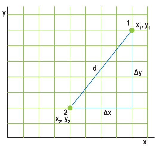
To describe the distance between any two points, which is invariant, we can write the complicated expressions above in a more compact and general way so that they are easier to understand. If we use the following notation:

\[Δx=x_1–x_2 \nonumber \]

\[Δy=y_1–y_2 \nonumber \]

for any two points 1 and 2, then we can write a much simpler expression for the distance, d, between them:

\[d^2=Δx^2+Δy^2 \nonumber \]

This is illustrated in Figure 9.8. Again we are using Greek Δ’s because we are talking about an interval. In this case, we mean changes in x and y.

Figure 9.8: Coordinate system with two points, 1 and 2, with a triangle shown to illustrate how the Pythagorean heorem is used to calculate their separation. Credit: NASA/SSU/Aurore Simonnet

DISTANCES AND COORDINATES

Worked Examples

1. Find the distance between the points (4, 5) and (8, 3).

• Given: (x₁, y₁) = (4, 5) and (x₂, y₂) = (8, 3)
• Find: d
• Concept: d² = Δx² + Δy² = (x₁ – x₂)² + (y₁ – y₂)²
• Solution:

Use the Pythagorean Theorem to find the distance squared. Then take the square root to find the distance.

d² = (4 – 8) ² + (5 – 3) ²
d² = (-4) ² + (2) ² = 16 + 4 = 20
d = (20)^1/2 = 4.47

The Graphing Tool, which is available in the tool bar, can help you to visualize where the points are in the coordinate system as you work through these problems.

For this example, our two points would be displayed as in Figure A.9.1.

Figure A.9.1: The points (4,5) and (8,3) are plotted using the Graphing Tool. Credit: NASA/SSU

For another example see Math Exploration 9.2.

Math Exploration 9.2

Questions:

Spacetime Diagrams

When Albert Einstein published his first paper on special relativity in 1905, he did not yet fully grasp its geometrical nature. He came to appreciate these aspects of the theory over the next several years while working with mathematician Hermann Minkowski (1864–1909). Minkowski developed the idea of spacetime , in which events occur in a four-dimensional space that includes both (the three dimensions of) space and (one more dimension of) time—hence, the name.

Spacetime is dynamic. You can plot the wanderings of a particle by tracing its path in this spacetime; i.e., you can plot its position at every moment in time. Such a path is called the worldline of the particle, and it traces out events in the life of the particle, both past and future. Events are just that. They might be the collision of the particle with another particle, or the moment the particle decays into other particles. In any case, the points in spacetime are called events, and a particle’s worldline is the string of events that comprise its existence, each tagged with a time and place of occurrence.

As a concrete example, you might describe some of the events in the worldline of your day with the following table:

EVENT	TIME	LOCATION	DESCRIPTION
1	6:00 AM	Bedroom	Get out of bed
2	6:05 AM	Bathroom	Take shower
3	6:30 AM	Kitchen	Have breakfast
4	7:00 AM	Front door	Leave for school
5	7:10 AM	Home bus stop	Board bus
6	7:45 AM	School bus stop	Arrive at school

Table 9.1: A sampling of events that might occur in your day. Other events might happen that we have not shown. These events might include getting dressed, brushing your teeth, sitting down on the bus, etc. A complete description of your day would include every event that occurred, including its time and location. In spacetime, these events link together in a continuous path.

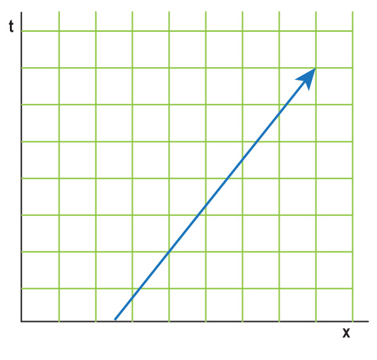
An event in spacetime has four coordinates, three in space and one in time: (t,x,y,z). However, spacetime plots are usually simplified by using only two axes: The vertical axis is time and the horizontal axis is space, as shown in Figure 9.9. We ignore the other two dimensions of space for the sake of convenience. Plotting all three spatial axes plus time would make the diagram too difficult to interpret. We cannot even imagine four perpendicular dimensions, let alone draw them on a two-dimensional piece of paper in such a way as to make sense of them. However, since we are free to choose a convenient coordinate system (as per the discussion above), we can take the direction of any particle’s motion to be only in the x-direction. We need only remember that the effects we encounter for the x-direction will also occur in y- and z- directions if there is motion directed along them.

Figure 9.9: In a spacetime diagram, the vertical axis is time. The horizontal axis is space, with only one of the axes shown for simplicity’s sake. All motion is taken to be only in this direction, again for the sake of simplicity. Credit: NASA/SSU/Aurore Simonnet

For a particle at rest, the plot is pretty boring. The particle has a constant position (x), so it is carried along a vertical path as time passes: Its worldline is a vertical line that intersects the x-axis at the position of the particle. An example is shown at left in Figure 9.10. Moving objects are only slightly more interesting. Their worldlines make an angle with the vertical, as the example on the right of Figure 9.10 demonstrates.

The slope of the worldline for a particle is related to its velocity. Specifically, since slope is rise over run, and velocity is distance over time, the slope of a particle’s worldline will be the reciprocal of its velocity, 1/v. This idea makes sense because a zero-velocity particle has a vertical worldline, i.e., one with infinite slope. As the particle moves faster, its worldline tips over more and more toward the horizontal because it travels farther in x in a given amount of time.

Figure 9.10: Worldlines on a spacetime diagram for a particle at rest (left) and for a particle moving at constant velocity (right). Credit: NASA/SSU/Aurore Simonnet

GRAPHING EVERYDAY SITUATIONS

In this activity, you will represent everyday physical situations in words, as data in a table, and as worldlines on a spacetime diagram. Assume the TV is at the origin of your spacetime graph. You will be using the Graphing Tool found in the toolbar.

1. Situation 1

2. Situation 2

3. Situation 3

So far, spacetime looks similar to Euclidean space, except that one of the axes is time. This difference is actually a pretty big one, if you think about it. Generally, in space, all directions use the same units of measure, feet or meters, for example. We never measure northward distances in inches and eastward distances in kilometers. We could do that, but it would not be very convenient because we could not easily compare the distance , say, between Paris and London, to that between Paris and Vienna (see Figure 9.11). The same is true in spacetime; things would be much simpler if we could use the same unit of measure along both axes.

Figure 9.11: A map of Europe showing Paris, London, and Vienna, with cardinal directions indicated. Distance from Paris to London: 13,296,371 in. Distance from Paris to Vienna: 1,037 km. Credit: NASA/SSU/Aurore Simonnet

Of course, one axis in spacetime is space and the other is time. Those are fundamentally different things. Still, it is easier to measure them using the same or at least similar units, and we have already been introduced to this idea. In previous chapters, we have used light-years. This is a unit of distance, not time; it is the distance light travels in a year. For example, light will travel 10 light-years in 10 years and 20 light-years in 20 years. Therefore, on spacetime diagrams, we will measure time in years (or hours, minutes, or seconds), and we will measure distances in light-years (or light-hours, light-minutes or light-seconds). This convention makes the two axes have related numerical values, greatly simplifying the comparison of distances along them.

Units of Time and Distance on Spacetime Diagrams

Worked Examples:

1. If we say that two events are 2 light-seconds apart, how much time does it take for light to travel between them?

If we say that two events are 2 light-seconds apart, it means that it takes light 2 seconds to travel from one to the other.

Since light travels 300,000 km/s, each light-second of distance is a very long way by terrestrial standards. If we want to convert back to meters or kilometers for some reason, we can always use the speed of light to do so, but it is more convenient just to use light-seconds or light-years to describe large distances.

2. If two events happen 2 seconds apart, how much time passes between them?

2 seconds. If we are talking about a time, not a distance, then the units have their usual meaning. An event that happens 2 seconds earlier than another event must happen before it.

Questions:

Given that we are using related units to measure both distance and time, we can immediately make an important inference about spacetime diagrams. In the units on our diagrams, light travels at a speed of one light-year per year. This means that its velocity is 1. If you are having difficulty understanding velocity in these units, it might be easier if you consider that our velocities are always in terms of the speed of light , c. So, in this way, they can be between 0 and 1. For example, a velocity of half of the speed of light would be 0.5. Since a photon has a velocity of 1, and the reciprocal of 1 is also 1, the worldline of a photon makes a 45-degree angle with the t- and x-axes. As we shall see, all massive particles must travel slower than light, so their worldlines all make an angle smaller than 45 degrees with the t-axis.

This is our first rule for creating and interpreting spacetime diagrams:

Rule 1. The worldlines of particles moving at the speed of light make a 45-degree angle with the t- and x-axes in a spacetime diagram. Worldlines of particles moving slower than light make an angle smaller than 45 degrees with the t-axis.

In the next activity, we will introduce you to the Spacetime Diagram Tool and practice drawing worldlines for particles traveling at various speeds.

SPACETIME WORLDLINES

Play Activity

Worked Example:

1. Use the Spacetime Diagram Tool to create worldlines for a particle moving with a speed of 0.5c.

To do this, adjust the “% speed of light” slider bar until it says 50%. The orange line will be the worldline for your particle. It should look like Figure A.9.3:

Figure A.9.3: Worldline for a particle moving at 0.5c in the Spacetime Diagram Tool. Credit: NASA/SSU

Questions:

A great power of spacetime diagrams is that they allow us to compare measurements of space and time in one reference frame to space and time in a different reference frame that is moving uniformly with respect to the first. To understand how this comparison is done, imagine two frames moving with constant velocity (that is, constant speed and direction) relative to one another.

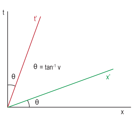
For an observer at rest in a frame with coordinates t and x, the spacetime axes are drawn perpendicular, as we have done In Figure 9.12. We can then plot the spacetime axes, t' and x', of a moving frame on the same diagram. To do this, we plot the t'-axis as a line with slope 1/v, where v is the relative velocity of the two frames. Why? First, we are free to take the origins of the two systems to coincide at t = 0 and t' = 0 (convenient coordinate systems again!). Then we can draw the worldline of the origin of the moving system in the system at rest.

Just as before, the worldline of a point moving at constant velocity makes a line with slope 1/v, and this result is exactly what the motion of the origin of the “primed” system will do in the spacetime diagram of the “unprimed” one. The worldline of the origin of the primed system must run along t' by definition, because x' = 0 for the origin and along the t'-axis. This reasoning gives us the location of our t'- axis in the (t,x) frame. Getting the x'-axis is a bit more complicated, but the x'-axis is a line with slope v. The details are described in Going Further 9.2: Finding the Location of the x'-Axis.

It turns out that the x'-axis makes the same angle with the x-axis as the t'-axis makes with t-axis. So, in the unprimed frame, the primed frame gets squeezed in toward the diagonal. The faster the relative velocity between the two frames, the more squeezed the primed frame becomes.

Figure 9.12: Axes (x,t) for a frame at rest with respect to an observer and, on the same diagram, axes (x',t') for a frame moving with velocity v. The angle between the t- and t'-axes and the x- and x'-axes are the same. They are the arctangent of the relative velocity between the two coordinate systems. Credit: NASA/SSU/Aurore Simonnet

Going Futher 9.2: Finding the Location of the X'-axis

To find the position of the x'-axis in the spacetime diagram, conduct the following thought experiment. Imagine that a flash of light is emitted from the point x' = 0 at some time t' = T < 0, or in other words, a flash of light is emitted from the origin of the primed system before it reaches the origin of the unprimed system. The flash is reflected and arrives back at x' = 0 at some time t' = T > 0. Because the return trip for the light is just the reverse of the outward trip, the time interval for the return trip ends T seconds after t' = 0. The geometry is shown in Figure B.9.1.

Figure B.9.1. A flash of light is emitted at event A, T seconds before t' = 0. It returns to its starting point at event C, T seconds after t' = 0. Event B, marking the reflection of the light, must lie on the x'-axis. Credit: NASA/SSU/Aurore Simonnet

Under these conditions, the reflection of the light must occur at t' = 0, and so that event, labeled event B, must lie on the x'-axis. Drawing a line from the origin through the reflection point locates the x'-axis.

Now we are ready for the second of our rules for creating spacetime diagrams:

Rule 2. To draw the time axis of a moving frame in the spacetime diagram of a frame at rest, draw a line with slope 1/v. To draw the spatial axis of the moving frame, draw a line with slope v.

In the next activity, we will use the Spacetime Diagram Tool to practice drawing axes for moving frames of reference.

SPACETIME AXES

Play Activity

Worked Example:

1. Use the Spacetime Diagram Tool to create axes for a reference frame moving with a speed of 0.5c.

• To create them, adjust the “% speed of light ” slider bar until it says 50%.
• The orange line will be the t'-axis.
• Click the “x'-axis” button to display the x'-axis (green) for the moving reference frame.
• Your diagram should look like Figure A.9.4.

Figure A.9.4: Axes for a reference frame moving at 0.5c, as drawn by the Spacetime Diagram Tool. Credit: NASA/SSU

Questions

We are almost ready to use our spacetime diagrams to begin exploring some applications of relativity and what relativity says about the world. However, we still need to know how to compare the scales on the primed and unprimed frames. It turns out that they are not the same. To understand why, we have to employ the invariance principle for spacetime. This principle is analogous to the invariance principle we encountered for Euclidean space, where points have an existence independent of the coordinates we choose to describe them. Any coordinate systems we use to describe the world do not affect the distance between points, nor the orientation of points to each other. Spacetime is the same as Euclidean space in this regard, but there is one critical difference. To understand this difference, recall that the invariance of Euclidean space is encapsulated by the Pythagorean theorem :

\[d^2=Δx^2+Δy^2 \nonumber \]

In spacetime, we have an analogous expression:

\[s^2=Δt^2−Δx^2 \nonumber \]

Here we have used the letter s instead of d to remind ourselves that we are not measuring a distance between points in space, we are measuring the separation between events in spacetime—an important distinction. And, just as the distance between two points does not depend on the Euclidean coordinate system used to describe them, so the separation of events in spacetime is independent of the coordinates used. Events have an existence all their own in spacetime, independent of the spacetime coordinates. This is our third rule for spacetime diagrams, but it is far more important than that—it is the essence of special relativity.

Rule 3. The spacetime interval between two events, as defined above, is independent of the coordinate system used to describe t and x. It is said to be invariant.

Notice the minus sign in the spacetime expression. This minus sign seems innocent enough, but it is responsible for the profound differences between the familiar properties of Euclidean space and the counterintuitive properties of spacetime. Also, because of the minus sign, it is possible for the spacetime interval, s², to be negative. But, that means that the spacetime separation, s, could be the square root of a negative number, or imaginary. What does that mean? We are not really sure, but we do not have to worry about it. It is really only the spacetime interval, s², that is important for our understanding of spacetime.

Going Further 9.3: Examining the Differences Between Euclidean Space and Spacetime

Consider one of the differences between Euclidean space and spacetime: The points in Euclidean space that are all equidistant from a given point make a circle around it, or a sphere, if we consider all three dimensions. This result makes sense. After all, the Pythagorean theorem is the same as the equation for a circle:

\[r^2=y^2+x^2\]

However, the equation for the spacetime interval has the same form as the equation for a hyperbola:

\[r^2=y^2−x^2 \nonumber\]

Apparently, spacetime intervals satisfy this equation, i.e., events that are equidistant from each other lie along hyperbolae! This is definitely not Euclidean. Figure B.9.2 compares Euclidean distances (on left) to spacetime intervals (on right). Note that we have used (x,t) coordinates for the spacetime plot instead of (x,y), in keeping with our convention that spacetime uses time as the vertical coordinate, while normal space uses y. As before, a spacetime interval is s, whereas d is used for a distance through Euclidean space.

Figure B.9.2. These graphs show points equidistant from the origin. In Euclidean space, at left, the points lie on a circle, with the origin at its center. In spacetime, events equidistant from the origin lie along a hyperbola, as shown at right. To be clear, all points along the hyperbola at right have the same spacetime separation from the origin, just as all points along the circle at left lie the same distance from the origin. Credit: NASA/SSU/Aurore Simonnet

While the points along a hyperbola in Euclidean space are not all the same distance from the origin, they are the same distance from the origin in spacetime. The fact that we are forced to make our plots on the Euclidean space of a flat computer screen or piece of paper obscures the true nature of the spacetime plot. Do not let the limitations of the presentation medium obstruct your understanding of how spacetime differs from Euclidean space in this vital way. All of the points along a given hyperbola in the spacetime plot have the same spacetime separation from the origin.

We can find the correct scale for the (t',x') axis for a moving frame (the space between adjacent ticks on the axis), by plotting these hyperbolae for integer values of s. The intersection of each hyperbola with the t'-axis gives the coordinate where t' = s. Why? Because along the t'-axis, the x'-coordinate is zero. The situation is the same as along the t-axis, where the x-coordinate is zero. To take a specific example, consider a hyperbola for s = 2. The intersection of that hyperbola with the t-axis is where t = 2, because along the t-axis, x = 0. So, we have s² = 2² = t² – x² = t² – 0², or t = 2. Along the t'-axis, x' = 0, so t'² – 0² = 2^2,, or in other words, t’ = 2. To find other values of t', you must simply find the intersection of the axes with the hyperbola for a given value of s. The spacings between ticks along the x'-axis are the same as those along the t'-axis.

The final thing we need to understand about spacetime diagrams has to do with reading the coordinates of an event in two different reference frames.

As an example, notice the event labeled A in Figure 9.13. In the unprimed system (the system in which the observer is at rest), the event occurs at position x = 8 and time t = 10. How can we tell? If you have ever read a graph, you know that you read off the x-coordinate by drawing a line through event A parallel to the t-axis. Lines parallel to the t-axis all have the same value of x, so by reading off the x-intercept of this line, you will determine the x-coordinate of event A. Similarly, to read the t-coordinate of A, draw a line through the event parallel to the x-axis.

In the primed system, which moves with velocity 0.5c relative to the unprimed, the coordinates of the event are x' = 3.5 and t' = 6.9. How can we read these coordinates? Read off the x'-coordinate by drawing a line through the event A and parallel to the t'-axis. Similarly, to read the t'-coordinate of A, draw a line through the event and parallel to the x'-axis. Lines parallel to the x'-axis all have the same t'-coordinate, which is to say they are simultaneous in the primed frame.

Figure 9.13: Spacetime diagram showing how to find the (x,t) and (x',t') coordinates of an event A. The yellow lines are parallel to the t- and x-axes. They can be used to read off the x and t coordinates for A. The red line is the t'-axis and the green line is the x'-axis. The blue lines are parallel to the t' and x' axes, so they can be used to read off the x'- and t'-coordinates for A. Credit: NASA/SSU/Aurore Simonnet

This is our last rule for building and reading spacetime diagrams:

Rule 4. The spatial coordinate of an event is found by drawing a line parallel to the time axis and finding its intercept with the space axis. The time coordinate of an event is found by drawing a line through the event parallel to the spatial axis and finding its intercept with the time axis. This works for both moving (primed) and rest (unprimed) reference frames.

Those are all the things you will need to know in order to interpret spacetime diagrams. Now, we will use what we have learned to explore how events will be described by observers in two different frames.

READING EVENT COORDINATES

In this activity, you will use the Spacetime Diagram Tool to create a graph similar to Figure 9.13.

Play Activity

Hit the Reset button on the tool, if you have not already.

The Spacetime Separation Between Events

Worked Examples:

1. Calculate the spacetime interval

(s²) between event A in Figure 9.13 and the origin in both the (a) unprimed and (b) primed reference frames, and (c) verify that s² is invariant.

(a) Answer:

• Given: x₁ = 8, x₂ = 0, t₁ = 10, t₂ = 0
• Find: s²
• Concepts: s² = Δt² – Δx², Δt = t₁ – t₂, Δx = x₁ – x₂
• Solution: Δx = 8 – 0 = 8, Δt = 10 – 0 = 10, s² = 10² – 8² = 100 – 64 = 36.0

(b) Answer:

• Given: x₁ = 3.5, x₂ = 0, t₁ = 6.9, t₂ = 0
• Find: s²
• Concepts: s² = Δt² – Δx², Δt = t₁ – t₂, Δx = x₁ – x₂
• Solution: Δx = 3.5 – 0 = 3.5, Δt = 6.9 – 0 = 6.9, s² = 6.9² – 3.5² = 47.6 – 12.3 = 35.3

(c) The spacetime interval, s², is the same in both cases (within rounding error), which means it is invariant.

Questions:

Understanding Event Coordinates

Recreate the diagram in Figure A.9.5 using the Spacetime Diagram Tool, and answer the following questions.

Figure A.9.5: Schematic shows events A, B, and C, with lines indicating how the coordinates of the three events are to be read in two different reference frames. To read the coordinates, the events must be plotted using the Spacetime Diagram Tool. Credit: NASA/SSU/Aurore Simonnet

Play Activity

In this section, we have introduced spacetime diagrams as a tool to help us understand the relationships between different events in spacetime and how observers in different frames view these events. In particular, the activities have illustrated that time and space coordinates of events can mix in unexpected ways when viewed from different frames of reference. For example, in the last activity, we saw that both the time and space parts of an event in one frame feed into the time part (or space part, for that matter) of the event as viewed in a different frame. That is why the time differences for the three events A, B, and C were not given by the simple time dilation equation. The next section puts these new tools and ideas to work to help us understand some of the weird results of special relativity.